

AlGaAs/GaAs Heterojunction Solar Cell Simulation: Device Structure, Band Alignment, J–V, EQE and Suns–Voc
1. Introduction: why use an AlGaAs/GaAs heterojunction?
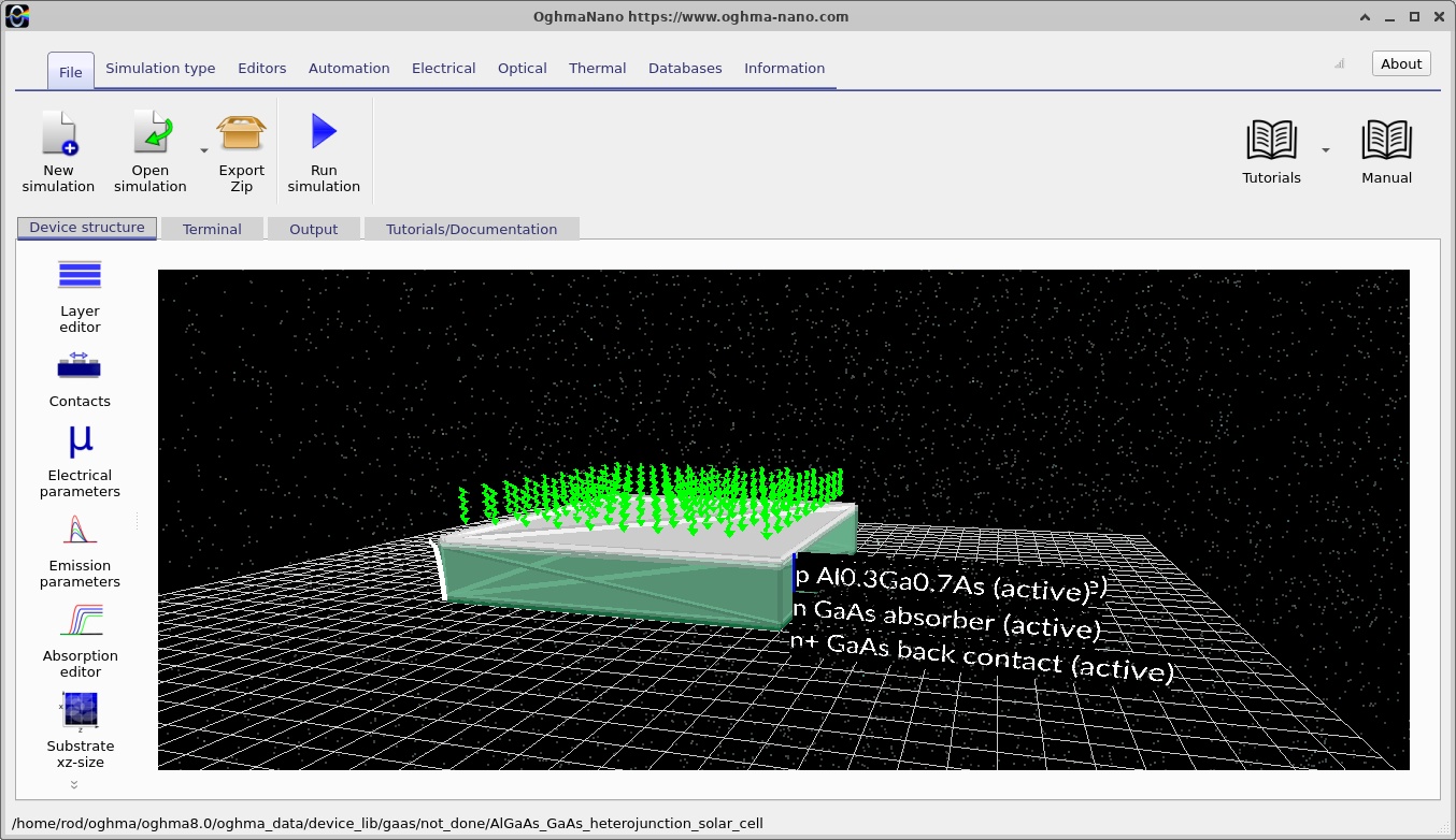
Gallium arsenide (GaAs) is a direct-bandgap III–V semiconductor widely used in high-performance photovoltaic devices. Its relatively strong absorption above its band edge allows a thin absorber to collect a substantial fraction of the incident sunlight at suitable wavelengths. A conventional GaAs homojunction, however, can suffer unwanted optical absorption and minority-carrier recombination close to the illuminated surface. A wider-bandgap semiconductor placed on the illuminated side can reduce these losses when its optical and electronic properties are chosen appropriately.
This tutorial models a p-type Al0.3Ga0.7As / n-type GaAs heterojunction. The top two AlGaAs layers form a wider-bandgap p-type window/emitter, while the underlying n-type GaAs provides the principal optical absorption region. The difference in bandgap and electron affinity across their interface introduces conduction- and valence-band discontinuities in addition to the electrostatic bending produced by ionised dopants. The resulting heterojunction must therefore be analysed using both the material band offsets and the carrier quasi-Fermi levels; treating it as a GaAs-only PN diode would miss important physics.
We will use OghmaNano's one-dimensional drift–diffusion solver coupled to an optical generation calculation. The supplied model includes an illuminated J–V sweep, options for EQE and intensity-dependent calculations, and saved internal profiles. The workflow is deliberately based on an already-configured example, so the goal is to understand, run and inspect the device rather than re-enter every parameter from scratch.
In a photovoltaic device, absorbed photons create electron–hole pairs; selective contacts extract the carriers and the resulting internal quasi-Fermi-level splitting produces an open-circuit voltage. A useful model must connect optical absorption and charge generation to junction electrostatics, carrier extraction and recombination. The sections below examine each of those links directly.
2. Creating the simulation from the GaAs demos
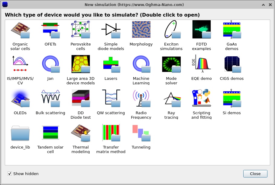
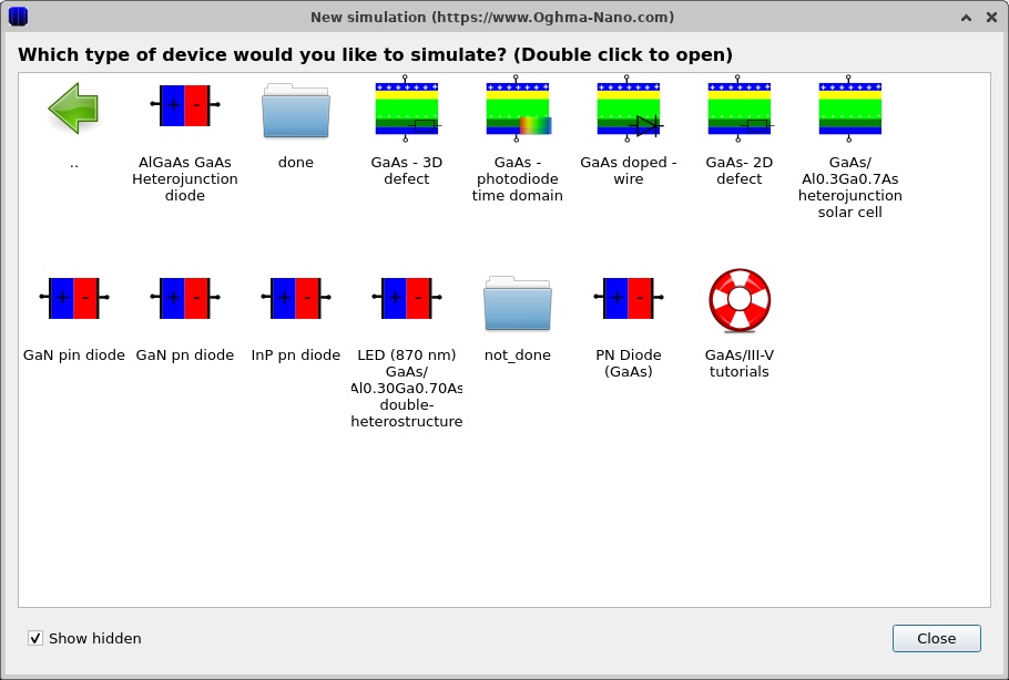
Open OghmaNano and select New simulation. In the simulation browser, open GaAs demos, then select AlGaAs/GaAs heterojunction solar cell. The selection dialog and demo category are shown in ?? and ??. The example opens in the main device-structure window (??).
The main window contains a three-dimensional graphical representation of the device. The physical simulation described here uses spatial variation along the y direction, normal to the layers. The rendered slab is therefore a way of seeing the stack and contacts rather than evidence of a full three-dimensional electrical solve. Select the Device structure ribbon to inspect or adjust the layers; the Output and Terminal tabs will be used after running.
It is useful to save a separate copy of the example before experimenting. Keep the baseline intact so that changes to doping, alloy fraction or interface parameters can be compared against a working reference.
3. Inspecting the epitaxial stack, doping and alloy composition
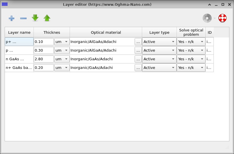
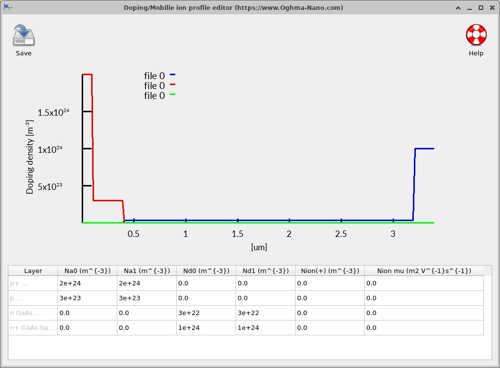
Open the Layer editor to examine the four epitaxial regions (??). The exact starting geometry and doping of this example are summarised below. All concentrations are expressed as volume densities in m−3, as stored in OghmaNano; to convert to cm−3, divide by 106.
| Layer, top to bottom | Thickness | Position from top | Majority doping | Physical role |
|---|---|---|---|---|
| p+ Al0.3Ga0.7As | 0.10 µm | 0–0.10 µm | NA = 2 × 1024 m−3 (2 × 1018 cm−3) | Highly doped front contact/window region |
| p Al0.3Ga0.7As | 0.30 µm | 0.10–0.40 µm | NA = 3 × 10²³ m−3 (3 × 1017 cm−3) | p-type wide-bandgap emitter |
| n GaAs absorber | 2.80 µm | 0.40–3.20 µm | ND = 3 × 10²² m−3 (3 × 1016 cm−3) | Main photon-absorbing and charge-collection region |
| n+ GaAs back contact | 0.20 µm | 3.20–3.40 µm | ND = 1 × 1024 m−3 (1 × 1018 cm−3) | Electron-selective rear contact region |
The heterointerface is at y = 0.40 µm, where the p-type AlGaAs emitter meets the n-type GaAs absorber. This is simultaneously a change in majority doping polarity and a change in semiconductor composition. In contrast, the 0.10 µm interface inside AlGaAs and the 3.20 µm interface inside GaAs are principally changes in doping concentration; those boundaries do not introduce a new material system.
Open Doping / Ions from the electrical controls (??). The graph should show the high acceptor density near the illuminated contact, the lower acceptor density through the remaining AlGaAs emitter, the donor-doped GaAs absorber and the more heavily doped GaAs rear contact. The sign change in net doping identifies the PN junction. Doping is not itself an optical absorption parameter; it enters Poisson's equation through the ionised space charge and affects conductivity, recombination and carrier collection.
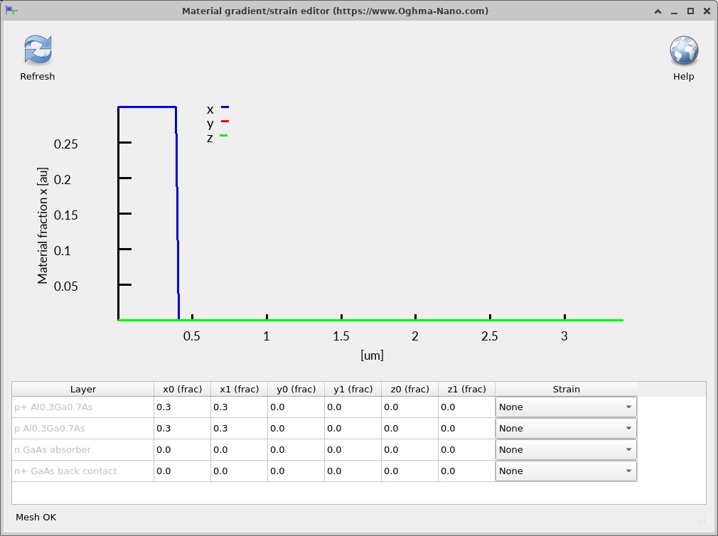
Next inspect Alloy composition (??). Both AlGaAs layers have g_x0 = g_x1 = 0.30: a constant aluminium fraction throughout their thickness. Both GaAs layers have g_x0 = g_x1 = 0 in this particular example. There is no composition grading in the supplied structure. A linearly graded AlGaAs region would require unequal composition endpoints and a Lua material model capable of evaluating the local composition at each mesh position.
The effect of the wide-bandgap window is wavelength-dependent. Photons with energies below the AlGaAs absorption onset can pass through the top semiconductor more readily, whereas photons above that onset may also be absorbed in the emitter. The magnitude of this benefit depends on the actual optical constants, layer thickness and internal collection properties; the Al fraction alone does not establish a quantitative reduction in front-surface losses.
4. Electrical material models and the heterojunction band offsets
Open the electrical parameter editor and inspect the Lua material scripts associated with the regions (?? and ??). This example evaluates the material parameters using the registered scripts, rather than setting every band parameter independently to a fixed value.
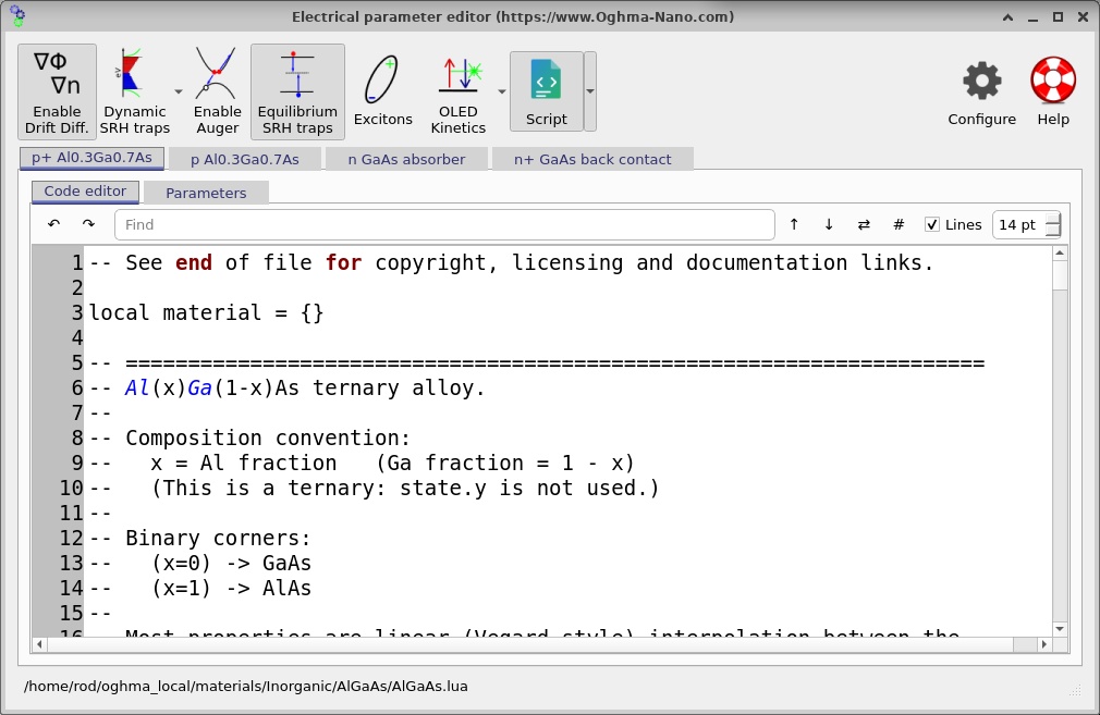
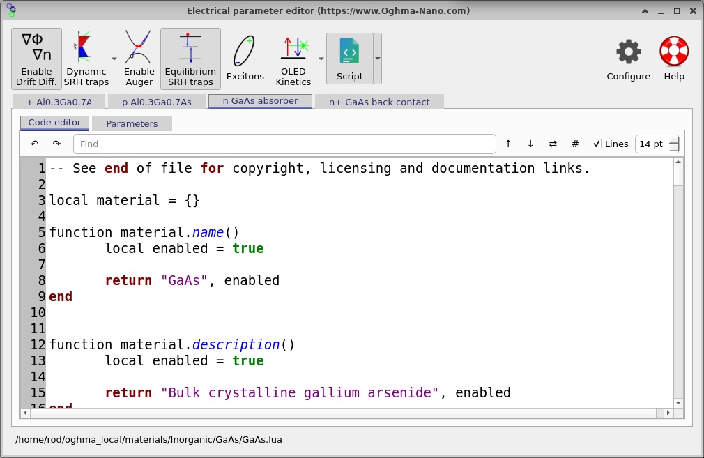
The AlGaAs and GaAs Lua paths are distinct: Inorganic/AlGaAs/AlGaAs.lua and Inorganic/GaAs/GaAs.lua. The top-layer composition value of 0.30 is available to the AlGaAs model, allowing composition-dependent electrical quantities to be calculated. The optical datasets are configured separately: Inorganic/AlGaAs/Adachi for the two AlGaAs layers and Inorganic/GaAs/Adachi for the GaAs layers. Electrical band parameters and optical refractive-index/absorption datasets should not be confused with each other.
At the heterointerface, the local conduction-band edge is related to the electron affinity by a convention of the form \(E_C=-\chi-q\phi\), and the valence-band edge by \(E_V=E_C-E_g\), provided that the same reference energy is used on both sides. The resulting discontinuities are conventionally written as \(\Delta E_C\) and \(\Delta E_V\). They depend on both the composition-dependent bandgap and the electron-affinity model. The greater bandgap of AlGaAs therefore does not, on its own, determine how the total offset is divided between the conduction and valence bands.
Physically, a conduction-band spike can impede electron extraction when sufficiently large, while an appropriate valence-band discontinuity can impede unwanted hole motion in the opposite direction. These effects compete with drift, diffusion, doping, thermal activation and recombination. This is why the simulated band structure is more informative than simply quoting a bandgap difference.
4.1. Transport and recombination parameters
OghmaNano solves the coupled Poisson and electron/hole continuity equations. In the drift–diffusion approximation, the electron and hole current densities depend on carrier mobility, carrier density gradients and the electrostatic field. In the usual sign convention, these can be expressed as
\[J_n=q\mu_n n\mathcal{E}+qD_n\frac{dn}{dy},\qquad J_p=q\mu_p p\mathcal{E}-qD_p\frac{dp}{dy}.\]The electric field and carrier populations are calculated self-consistently. Under illumination, the continuity equations must additionally account for photogeneration \(G\) and recombination \(R\). For example, with the usual one-dimensional current convention, \(dJ_n/dy=q(R-G)\) and \(dJ_p/dy=q(G-R)\) in steady state. Their sum should consequently remain spatially constant in an ideal steady-state solution without an additional distributed charge-storage term.
The JSON enables steady-state SRH recombination (ss_srh_enabled = "True") and gives a nominal mid-gap trap energy, trap density \(N_t=5\times10^{19}\,\mathrm{m}^{-3}\), and capture cross-sections \(\sigma_n=\sigma_p=10^{-22}\,\mathrm{m}^2\) in each layer. These fields describe the configured defect model; whether a field is taken directly from JSON or recomputed by the chosen material script must be checked against the effective values reported by OghmaNano. The rate of a standard one-level SRH process is
In a direct-gap semiconductor, radiative free-electron–to–free-hole recombination can also be important, conventionally represented by \(R_{\mathrm{rad}}=B(np-n_i^2)\). The program may also provide Auger coefficients and other channels through the material models. Do not infer which mechanism dominates merely from the presence of its settings: use the plotted recombination files, the actual enabled switches and the material-model values in the running example. For this device, the appropriate interpretation is obtained by comparing rates on the same voltage point and consistent vertical scales.
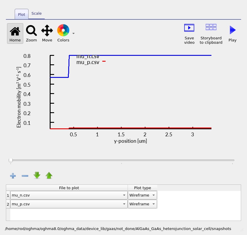
The electrical-editor view can be used to inspect mobility and other local properties (??). When experimenting with compositions, leave bandgap and electron-affinity database overrides disabled unless there is a specific reason to override the Lua values: manually fixed \(E_g\) or \(\chi\) can accidentally remove the intended composition dependence.
5. Electrical contacts and the simulation mesh
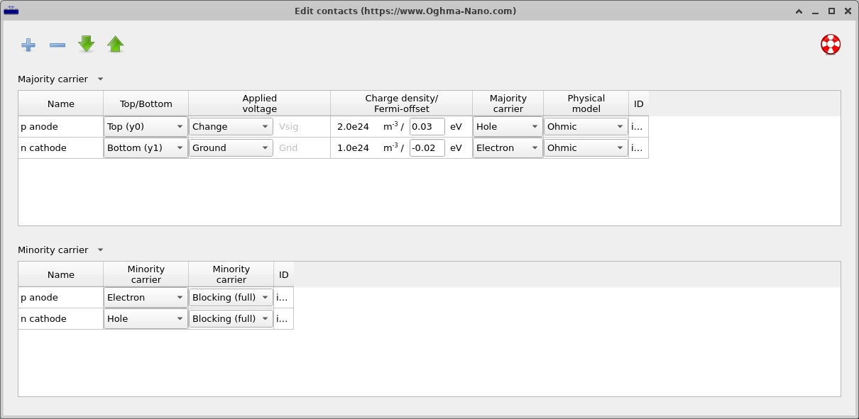
The model has two external electrical terminals. The upper p anode, at y0, is the driven contact; the lower n cathode, at y1, is the grounded terminal. Both use an ohmic majority-carrier boundary and a blocking minority-carrier boundary. This is an important modelling choice: the structure is not represented by generic symmetric contacts that extract electrons and holes indiscriminately. Open the contacts editor to see the contact rows (??).
At the anode the majority carrier is the hole and the minority carrier is the electron. The roles are reversed at the cathode. An applied sweep therefore changes the potential at the p terminal with respect to the grounded n terminal. The contact model is distinct from the highly doped epitaxial contact layers, which are part of the semiconductor geometry. The explicit terminal conditions determine how carriers leave the computational domain.
The electrical solver is configured for a one-dimensional y mesh. Its four mesh segments track the four epitaxial thicknesses with nominal point counts of 10, 17, 156 and 11, respectively. This is approximately 194 specified points, although the number of unique nodes actually used can depend on the solver's handling of shared boundaries. Both lateral electrical mesh directions are disabled. The mesh settings are visible in ??.
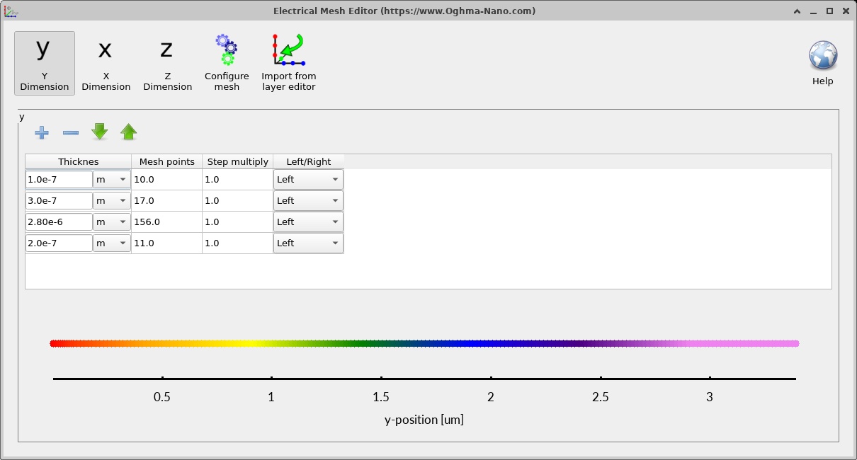
Mesh resolution matters especially close to the heterointerface at 0.40 µm, where electrostatic bending and band offsets may vary over a short distance. If the calculated band discontinuity or carrier density develops a narrow spike, a mesh-convergence check is more convincing than simply accepting the default trace. Repeat a calculation with a finer emitter/junction mesh and compare the J–V results as well as the relevant spatial profiles. If these change materially, the baseline mesh was not yet sufficiently resolved.
6. Running the illuminated J–V simulation
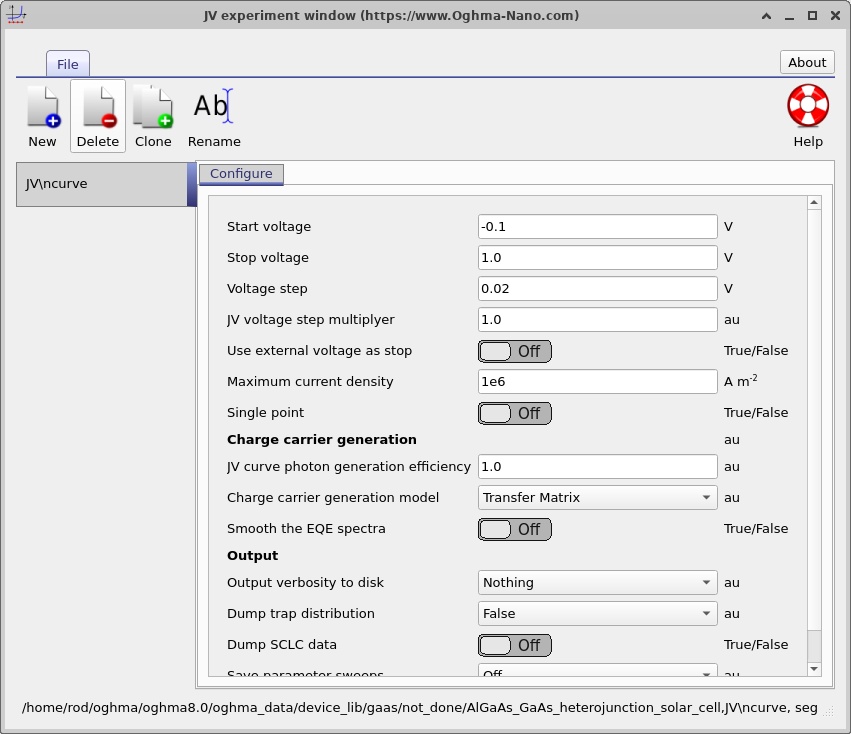
The default selected mode in the supplied configuration is J–V. Its voltage sweep is configured from −0.10 V to +1.00 V in steps of 0.02 V. Illumination uses an AM1.5G spectrum and the baseline light-source intensity scale is one sun (Psun = 1). Optical generation is coupled into the electrical simulation via the configured transfer-matrix generation model. The temperature set point is 300 K.
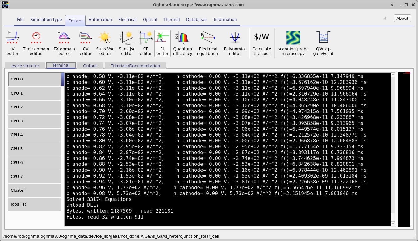
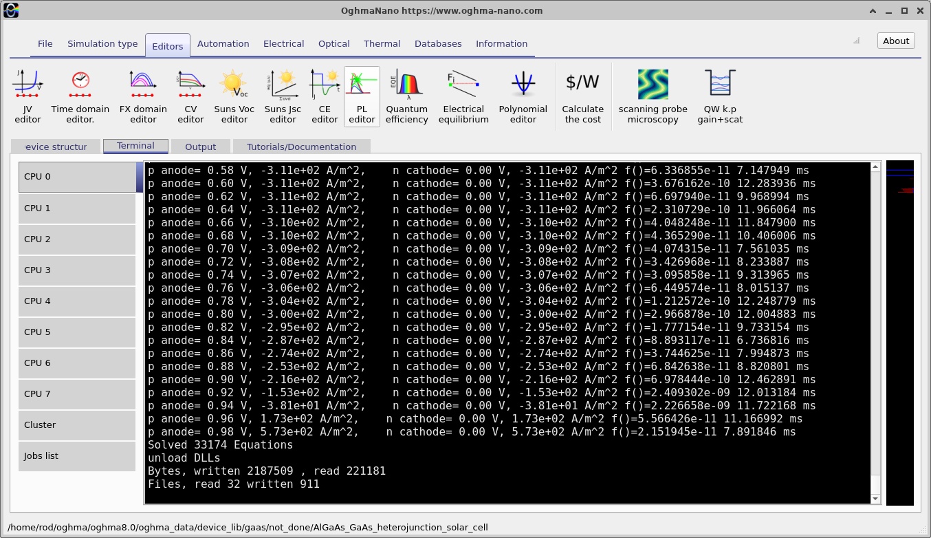
Before running, examine the Output tab (??). Click Run simulation. The Terminal tab displays progress and solver output; the paired terminal screenshots (?? and ??) show an early and a later state of the calculation. A changing terminal display is evidence that the solver is working, but it is not by itself proof that every point has converged. Check for completion, errors and the resulting output files.
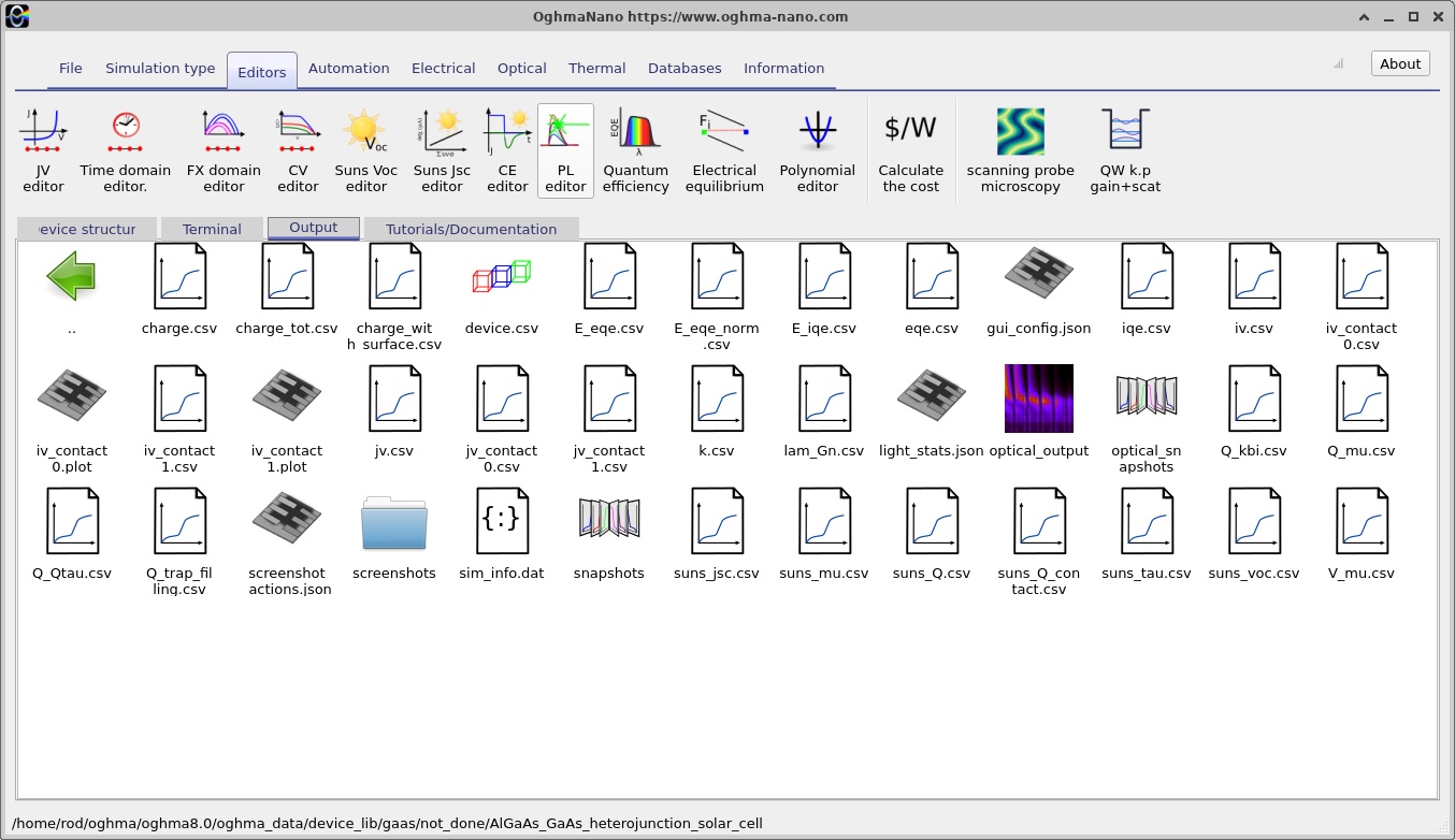
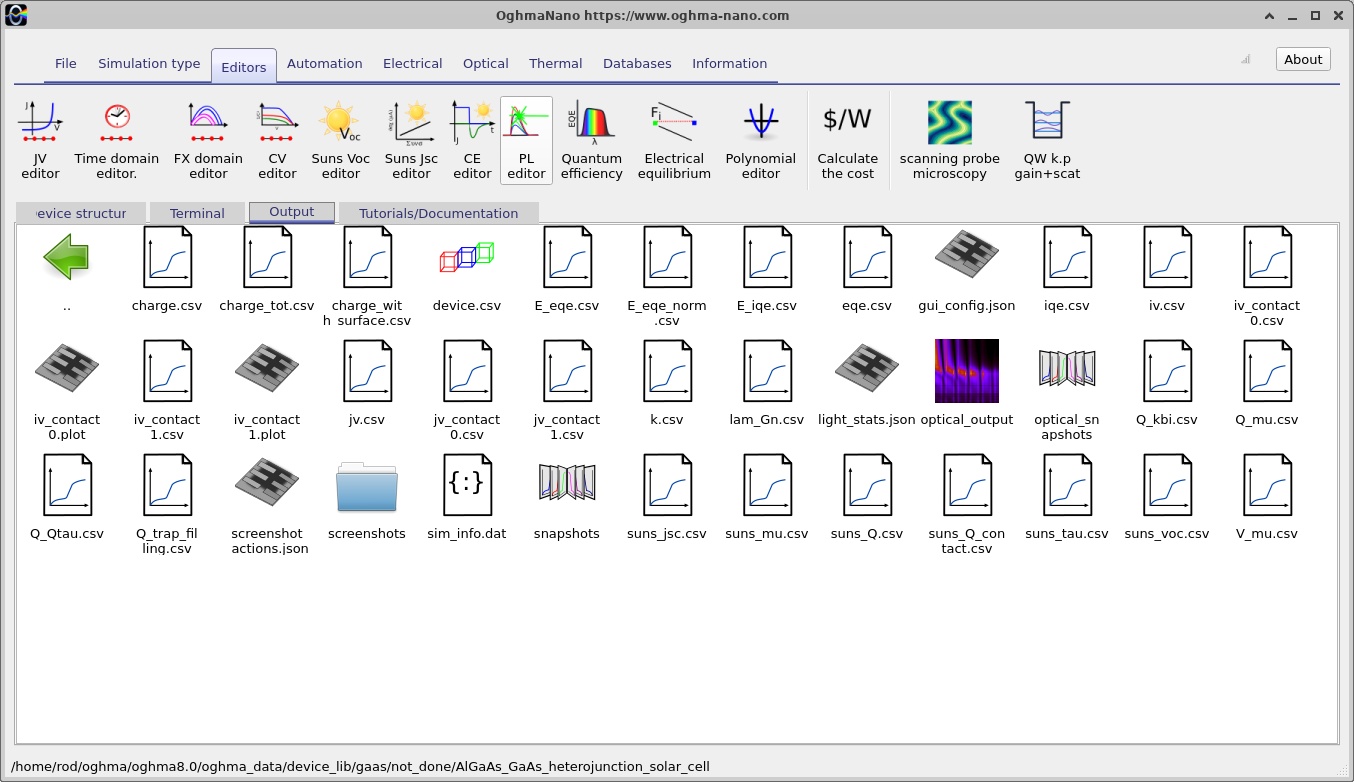
After execution, return to Output and open jv.csv (??). The illuminated J–V curve differs conceptually from the forward-bias dark diode curve. A simple first-order expression is \(J(V)=J_{\mathrm{dark}}(V)-J_{\mathrm{ph}}(V)\), for a sign convention in which extracted photocurrent is negative. The simulator's plotted sign follows its configured contact convention, so the physically meaningful quantities should be identified from the voltage and current intercepts rather than assuming every photovoltaic plot is drawn with the same signs.
The short-circuit current density, \(J_{SC}\), is the current density at \(V=0\), whereas the open-circuit voltage, \(V_{OC}\), is the voltage at which the terminal current density is zero. The maximum power point occurs at the applied bias that maximises the magnitude of power delivered to an external load, and the fill factor is defined by
\[FF=\frac{|J_{\mathrm{mpp}}V_{\mathrm{mpp}}|}{|J_{SC}|V_{OC}}.\]With consistently specified incident optical power density \(P_{\mathrm{in}}\), the conversion efficiency follows as \(\eta=|J_{\mathrm{mpp}}V_{\mathrm{mpp}}|/P_{\mathrm{in}}\). Do not report an efficiency simply from the curve's shape: it also requires the illumination power convention and a reliable identified maximum-power operating point.
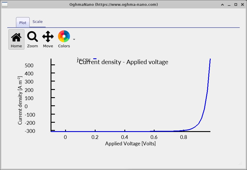
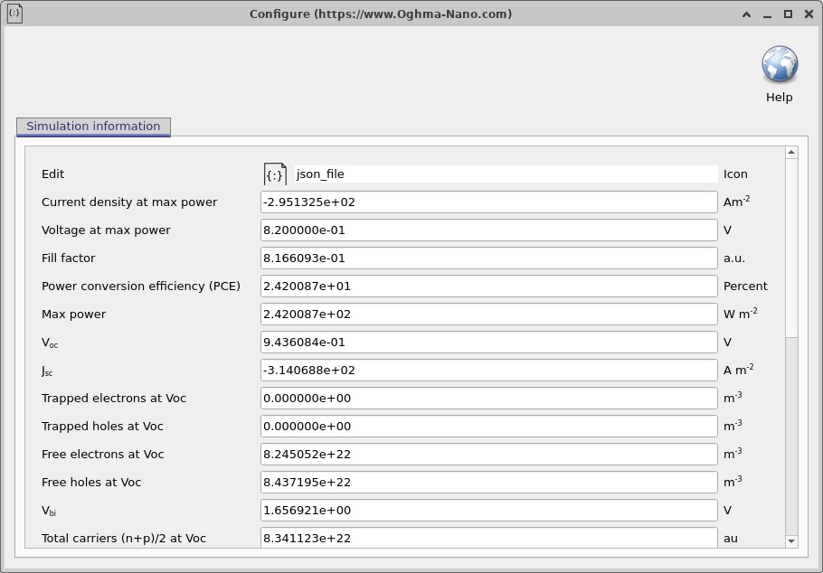
The J–V curve is the easiest performance summary, but it does not explain why a current is lost. A decrease in photocurrent can arise from inadequate absorption, poor carrier collection or increased recombination; a lower open-circuit voltage can result from stronger recombination or altered junction electrostatics. For that reason, the next sections use spatially resolved data as diagnostic evidence rather than relying on the J–V plot alone.
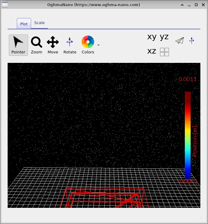
The device.csv visualisation (??) provides a useful independent check that the simulated physical regions and their boundaries correspond to the intended geometry. The Simulation information panel (??) is useful when comparing runs and checking the settings associated with a result.
7. Band diagrams, carrier densities and transport through the heterojunction
Open the saved snapshots from the output viewer and move the snapshot slider through the bias points. The four screenshots of each quantity below show different saved states from the same calculation; their numerical scales and bias labels should be read directly from the corresponding viewer. When comparing two states, first establish whether they share the same axis limits and which plotted quantity is being compared.
7.1. Conduction and valence bands, Fermi levels
The band diagram is the clearest place to identify the AlGaAs/GaAs heterojunction (??–??). The material interface is located at 0.40 µm. An abrupt change in the local band edges there reflects the material offset, whereas the smoothly varying curvature elsewhere reflects electrostatics. This distinction is central: a heterojunction cannot be interpreted solely in terms of a continuously bent GaAs bandgap.
At thermal equilibrium the electron and hole electrochemical potentials coincide, giving a common Fermi level. Out of equilibrium, the electron and hole quasi-Fermi levels may separate. Their difference is a measure of local carrier nonequilibrium and is related to the local product of electron and hole populations. At open circuit, the terminal voltage reflects the difference between the electrochemical potentials established at the selective contacts; one should not equate a single local quasi-Fermi-level separation at an arbitrary depth with the measured open-circuit voltage.
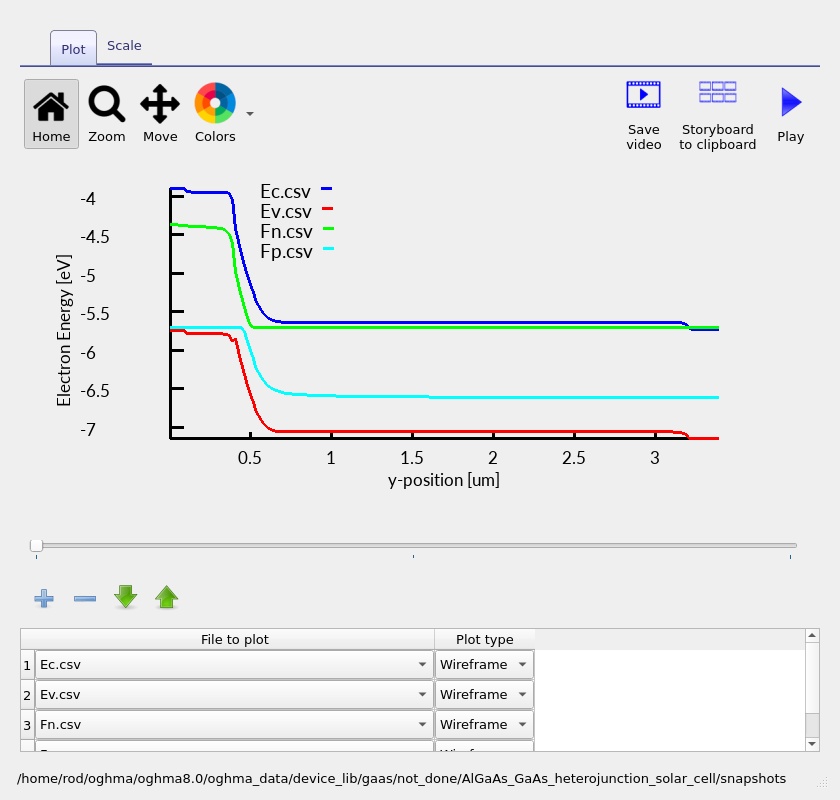
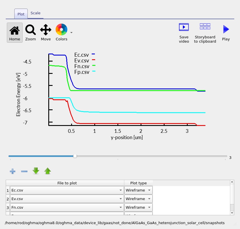
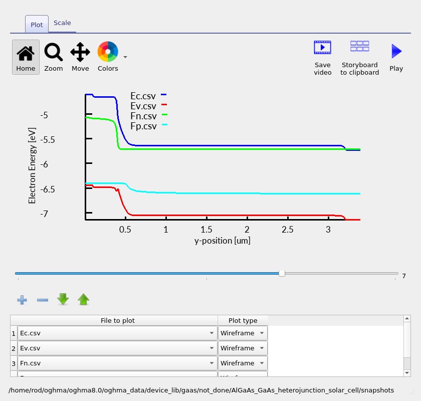
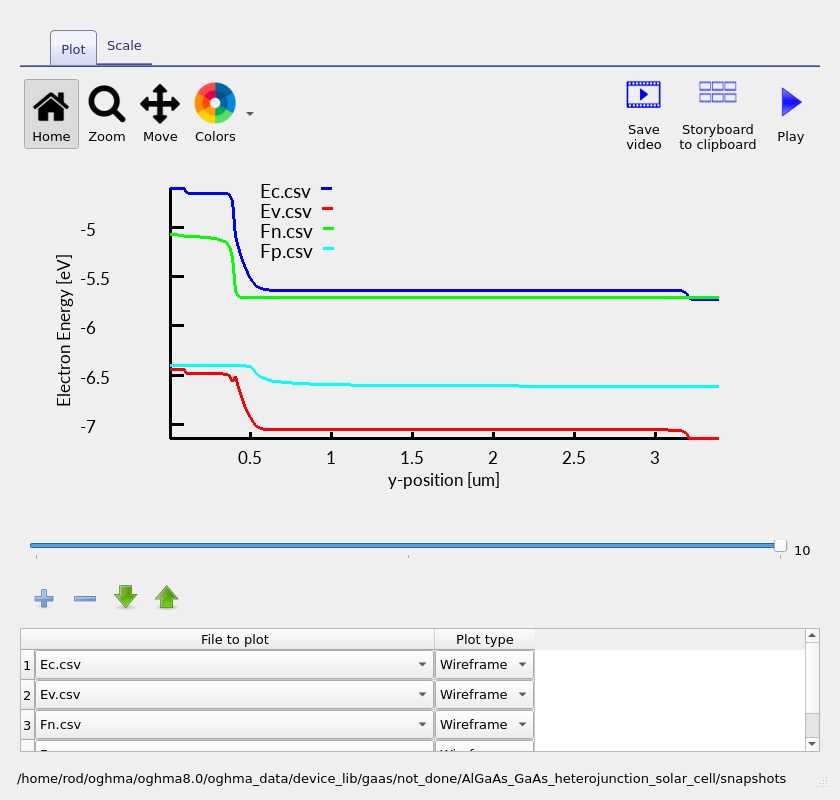
As the applied bias changes, the electrostatic potential and carrier distributions respond together. Under forward electrical bias, the junction barrier is reduced relative to equilibrium; under photovoltaic operation, photocarriers establish nonequilibrium populations and a photovoltage. Any apparent step in a quasi-Fermi-level trace should be examined alongside current flow and mesh resolution before being interpreted as a physically abrupt electrochemical potential.
7.2. Electron and hole densities
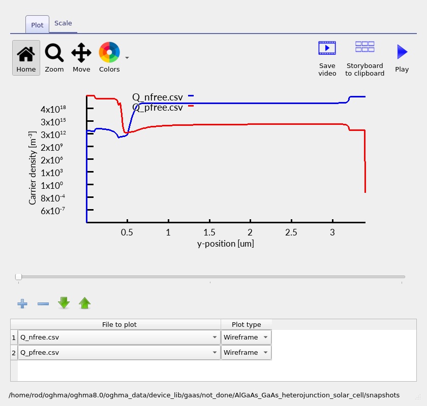
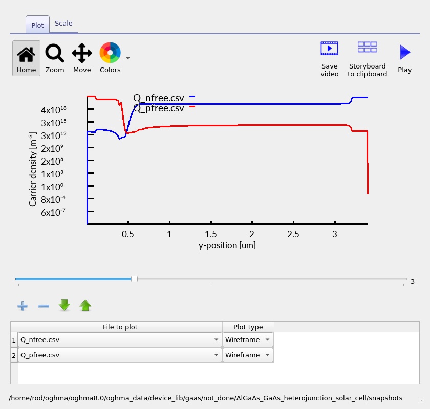
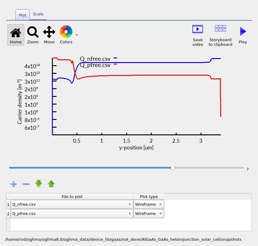
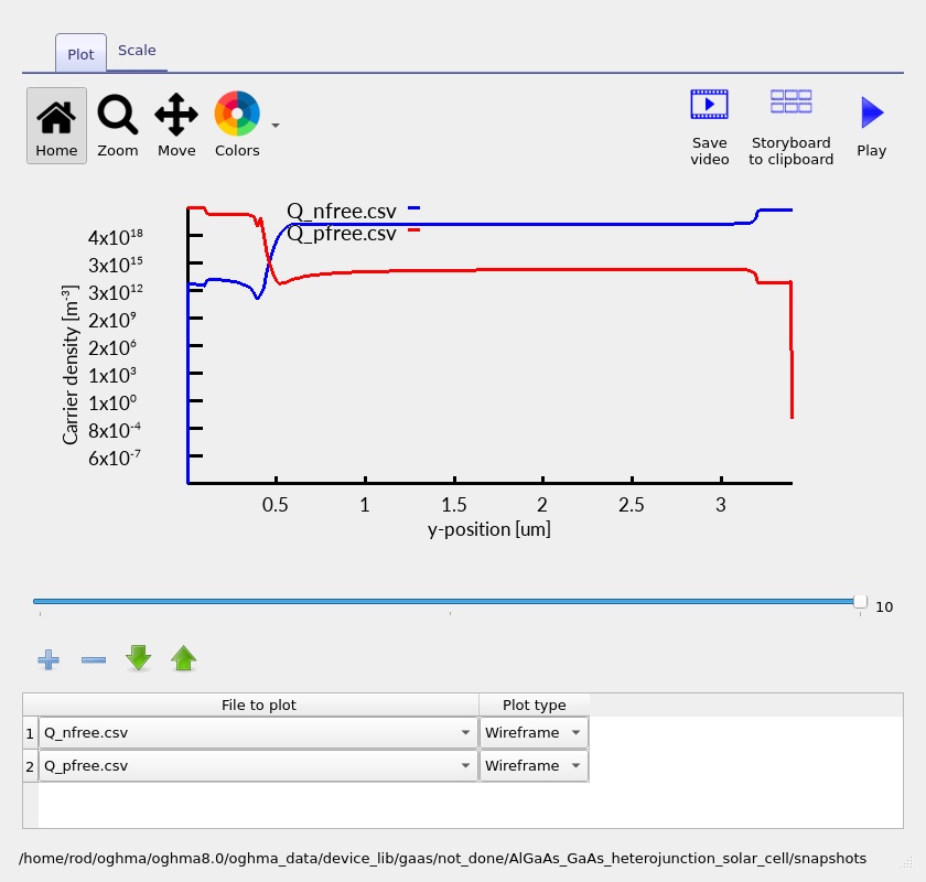
The carrier-density plots (??–??) distinguish majority-carrier regions from injected or photogenerated minority carriers. Through the p-type emitter the equilibrium majority species is holes; throughout the n-type absorber it is electrons. The minority-carrier profiles carry important information about collection and recombination, particularly on the GaAs side of the junction.
The electron and hole concentrations are sensitive to the effective density of states, band offsets, electrostatic potential and generation/recombination balance. Concentration changes cannot therefore be assigned exclusively to the doping profile. A steep change near the heterointerface can result from the combined effects of the local band alignment and drift–diffusion transport.
7.3. Electron and hole current densities
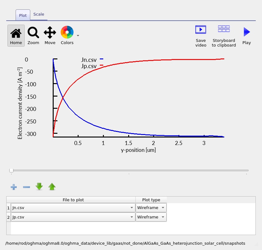
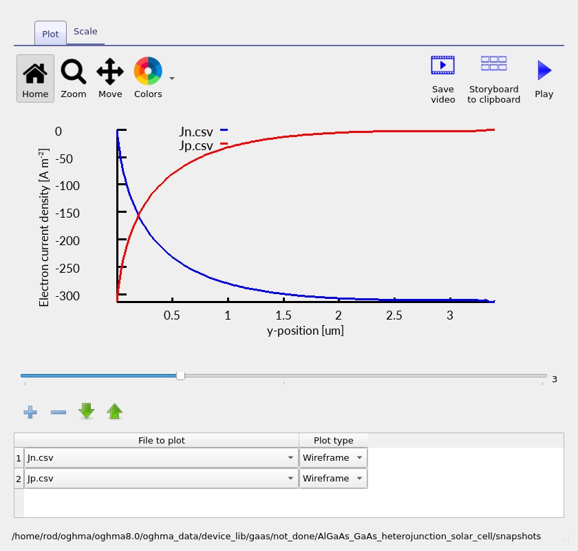
The electron and hole current plots (??–??) show how the total terminal current is partitioned between the two carrier types as a function of depth. Photogeneration creates both electrons and holes, but the way each species contributes to the current changes through the device according to its local generation, recombination, mobility and electric field.
In a steady-state one-dimensional calculation, the sum of the signed electron and hole currents should be constant away from any explicitly modelled distributed current source or loss. Each component, however, need not be constant: as carriers are generated and recombine, the electron and hole current components exchange contributions while maintaining the total current. This is a powerful consistency check for a completed solution.
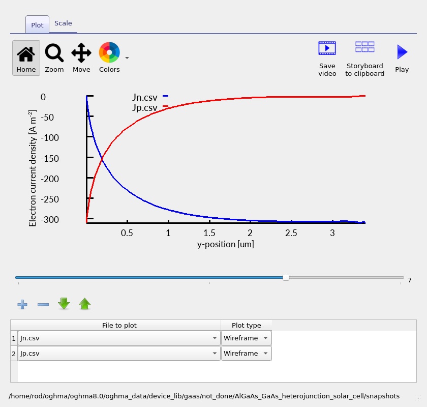
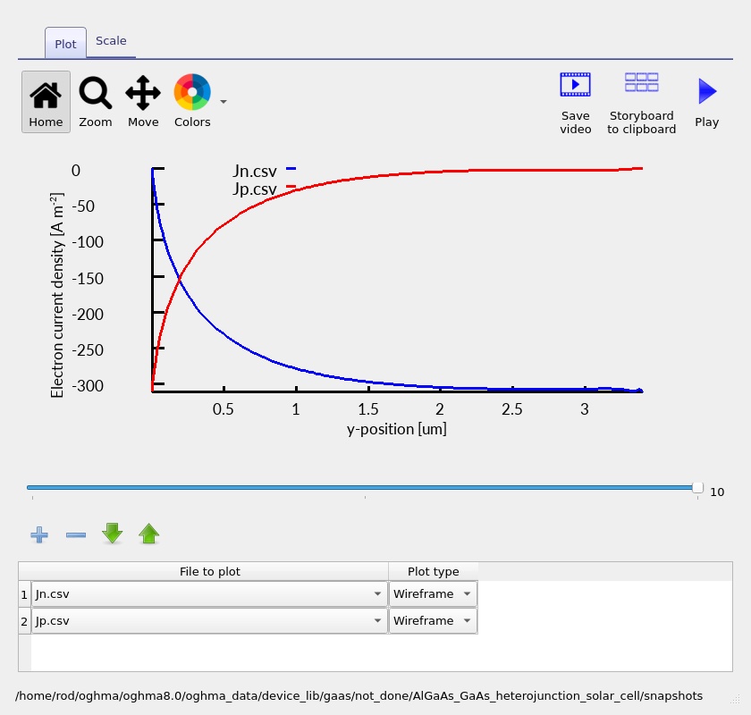
Some plots can appear particularly sharp near low-current conditions. Avoid diagnosing a physical transport barrier from a single noisy trace: inspect the band edges, carrier densities and the signed current components together, and check whether the feature changes when the mesh is refined. The separate mobility plot (??) provides a convenient way to see the modelled local transport coefficients and whether they vary with material or composition.
8. Recombination, carrier rates and photogeneration
Solar-cell current is the result of a competition between generation and loss. Photons absorbed in the device create carriers, but only a fraction of those carriers may reach the selective contacts. The local electron and hole continuity equations capture this balance. OghmaNano exposes a range of output rates, which can be compared spatially rather than only through a device-integrated current.
8.1. Recombination versus applied bias
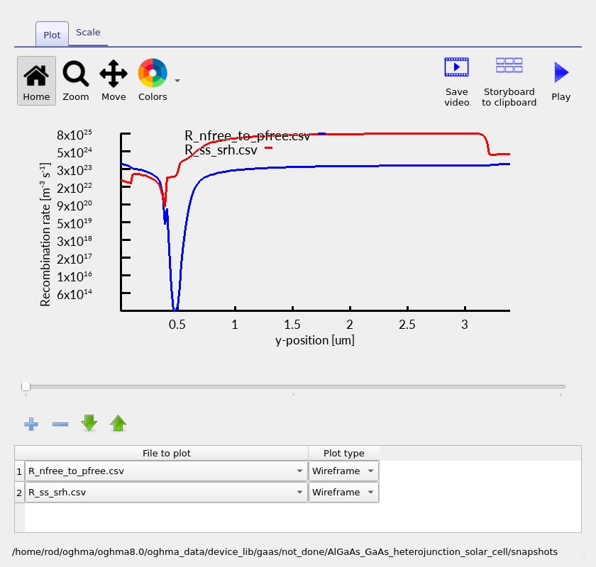
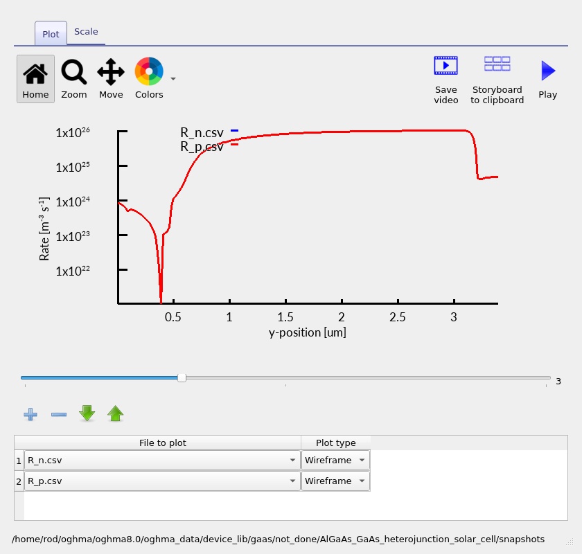
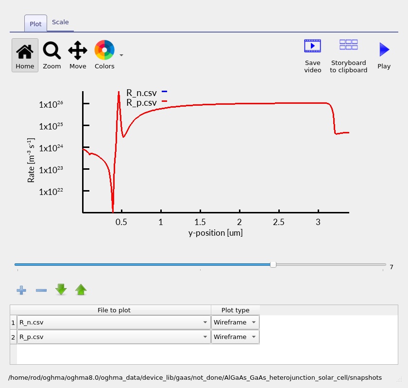
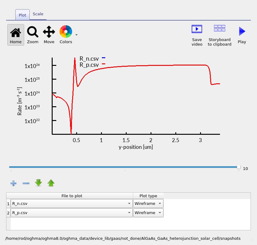
Open the recombination profiles (??–??). A recombination rate is a volume rate, usually expressed in carriers per cubic metre per second; it should not be compared numerically to a current density without integrating over a distance and multiplying by the elementary charge. For a one-dimensional device, an illustrative recombination-current density is \(J_{\mathrm{rec}}=q\int R(y)\,dy\), subject to the chosen definition of the net rate and boundaries.
Compare not only the peak heights but also the width and location of the rates. A spatially narrow high peak may contribute less to an integrated loss than a modest rate extending across the whole absorber. Use the same voltage and region when comparing mechanisms. In a heterojunction, carrier accumulation near a band offset may locally increase recombination, but the relevant diagnostic is whether such accumulation is actually visible in the density and band plots.
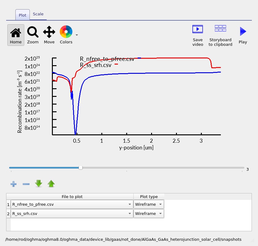
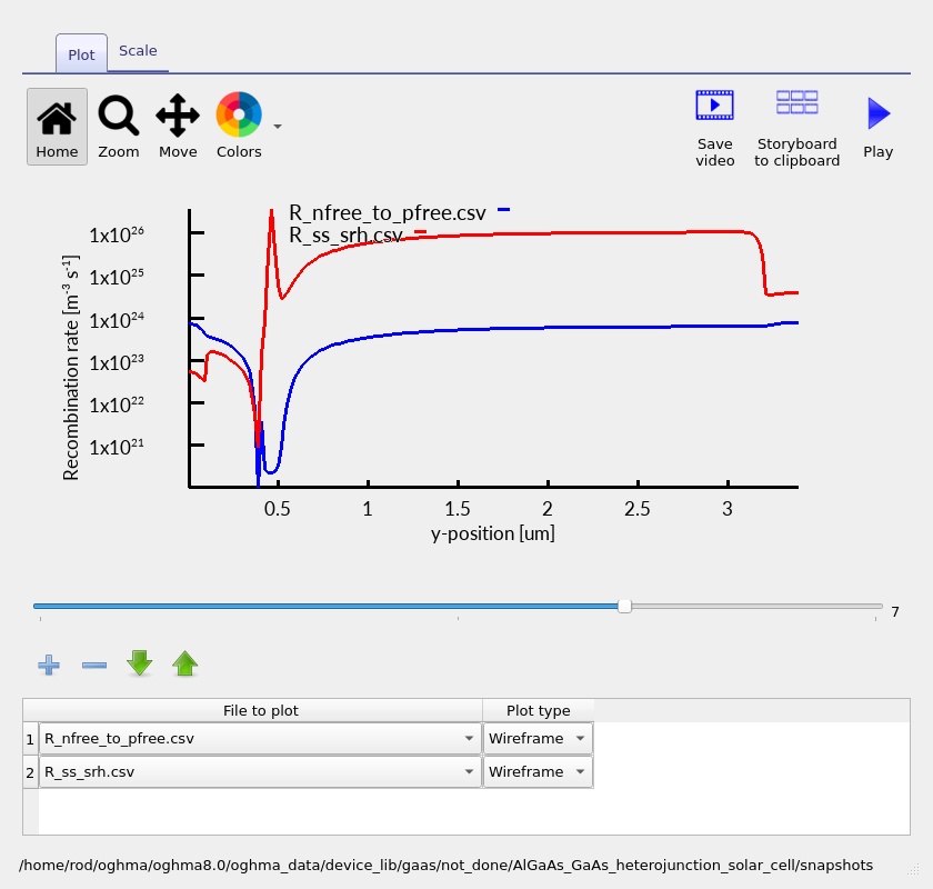
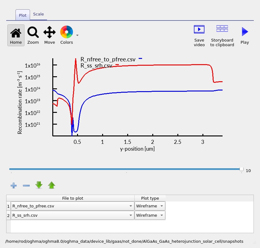
8.2. Electron–hole rates
The related electron–hole-rate outputs (??–??) help compare the rate terms shown by the snapshot viewer. It is important to distinguish net recombination from any individual capture, emission, generation or free-carrier transition rate. Not every plotted rate is necessarily an independent loss mechanism; summing displayed curves without checking their definitions can double-count transfer pathways.
For a net radiative recombination channel, the familiar law \(R_{\mathrm{rad}}=B(np-n_i^2)\) illustrates why recombination grows as both carrier populations increase. SRH recombination instead depends on trap occupancy and capture kinetics. The relative size of these processes depends on the effective material parameters in the run. This tutorial does not assume that radiative recombination dominates all layers or bias points merely because GaAs is a direct-gap semiconductor.
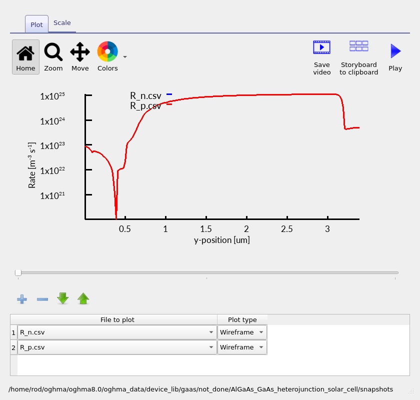
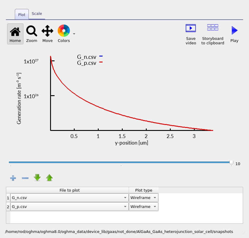
8.3. Generation profile
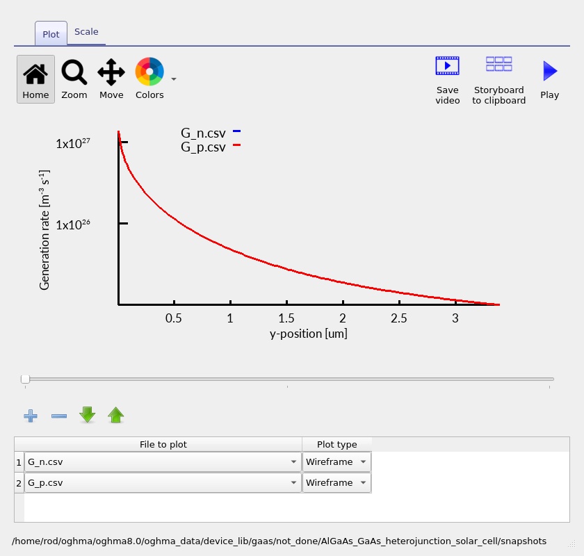
The optical carrier-generation rate is fundamentally different from a recombination rate: it is a source rather than a loss. For wavelength-dependent photon flux \(\Phi(\lambda,y)\) and absorption coefficient \(\alpha(\lambda,y)\), a simple local relationship is \(G(y)=\int \alpha(\lambda,y)\Phi(\lambda,y)\,d\lambda\), with the precise calculation depending on interference, reflection and the field definitions of the chosen optical model.
The saved generation profiles (?? and ??) allow you to see where photocarriers are produced. Stronger generation near the illuminated side can follow from exponential absorption; interference and wavelength-dependent absorption can produce a more complex depth dependence. An optically generated carrier is not automatically a collected carrier, which is why generation must be examined together with the current and recombination plots.
9. External quantum efficiency: wavelength-dependent carrier collection
External quantum efficiency (EQE) measures the number of electrons collected through the external circuit per photon incident on the device at a specified wavelength, subject to the sign and normalisation used by the output. In an ideal one-electron-per-photon collection picture, \(EQE(\lambda)=J_{\mathrm{photo}}(\lambda)/(q\Phi_{\mathrm{incident}}(\lambda))\), with the spectral current and photon flux expressed consistently.
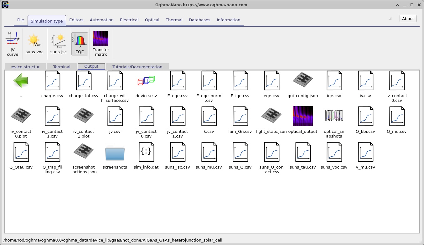
To open the EQE calculation, select the EQE simulation option in OghmaNano and run it, then examine its saved result under Output (??). The supplied simulation file also contains a configured EQE test wavelength of 710 nm; this setting should not be mistaken for a complete, measured or calculated broadband EQE spectrum unless a wavelength sweep has actually been performed and the output contains that spectrum.
For GaAs, photon energies near and above its bandgap correspond to the near-infrared/visible edge of photovoltaic response. The wider-bandgap AlGaAs emitter can be more transparent over part of the useful GaAs absorption range, increasing the fraction of light available to the absorber. At very short wavelengths, absorption in the front AlGaAs and recombination of carriers generated close to the surface may reduce collection. At longer wavelengths near the GaAs absorption edge, incomplete absorption in a finite-thickness 2.8 µm absorber can become important. Quantitative spectral conclusions should be drawn from the calculated EQE curve and verified optical datasets, not guessed from a bandgap alone.
EQE is not equivalent to optical absorptance: absorption counts photons absorbed; EQE counts collected carriers. Comparing them reveals electrical collection loss. If absorption is high but EQE is low at a particular wavelength, inspect the spatial generation profile and the recombination/transport behaviour of the layer in which those photons are being absorbed.
10. Suns–Voc and Suns–Jsc illumination-intensity calculations
10.1. Suns–Voc
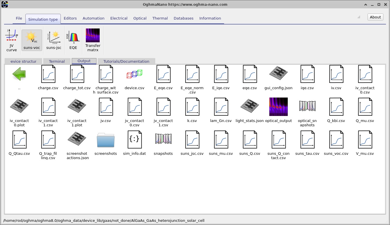
Suns–Voc probes the dependence of open-circuit voltage on illumination strength. Open circuit is defined by zero net external terminal current, so the photogenerated carriers build up a voltage instead of delivering power to a load. The supplied example contains a Suns–Voc configuration spanning an intensity multiplier from 0.01 to 1000 suns using multiplicative steps of 1.2. Access this simulation mode and inspect its output selection (??) and curve (??).
In an idealised diode model with approximately illumination-independent recombination physics, the relation \(V_{OC}\approx(n_{\mathrm{id}}k_BT/q)\ln(J_{\mathrm{ph}}/J_0+1)\) predicts a roughly logarithmic increase in open-circuit voltage with light intensity. Here \(n_{\mathrm{id}}\) is an effective ideality factor. In a heterojunction device, the local carrier distribution, band offsets, recombination channels and high-injection behaviour may all change with intensity, so the effective slope need not be constant over the entire sweep.
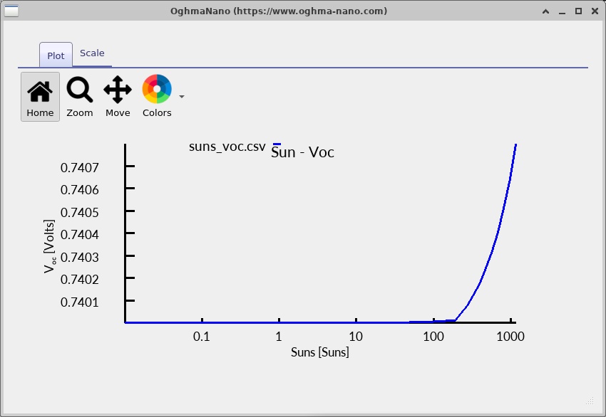
Suns–Voc is valuable for investigating the implied diode response under zero current. It does not by itself include all of the voltage losses caused by current flowing through a resistive contact or transport layer under power-generating conditions. A comparison of Suns–Voc behaviour with the illuminated J–V curve can therefore help separate recombination-related limitations from current-dependent transport losses, although interpreting such a difference requires consistency of illumination, recombination models and voltage definitions.
10.2. Suns–Jsc
Suns–Jsc examines short-circuit current versus illumination strength. The example is configured for a sweep starting at 0.01 suns and stopping at 10 suns, with a multiplicative intensity factor of 1.05 and the stored starting increment sundp = 0.01. Use the Suns–Jsc simulation selector and inspect the result in ?? and ??.
In the simplest constant-collection-efficiency regime, short-circuit current scales approximately linearly with the incident photon flux, so \(|J_{SC}|\propto P_{\mathrm{sun}}\). A systematic departure from linearity can indicate intensity-dependent carrier collection, recombination or transport. However, the interpretation should also account for the way the code changes its optical illumination scaling and the numerical convergence of each point.
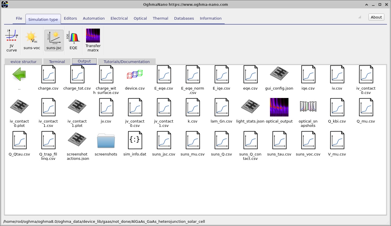
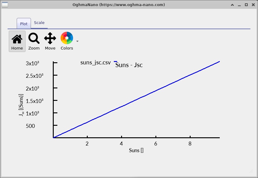
The two intensity sweeps answer complementary questions: Suns–Voc looks at the voltage established without external current, while Suns–Jsc looks at the collected current at approximately zero applied voltage. They should be interpreted alongside the ordinary one-sun J–V curve, not as substitutes for it.
11. Optical modelling and the spatial photogeneration distribution
The electrical solver requires a spatial photogeneration rate, but this rate is supplied by the optical calculation. In the present example the light source is configured for the AM1.5G solar spectrum, incident from the top (y0) side, and the generation model is transfer matrix. The spectral mesh spans 320–1100 nm with 201 configured wavelength points; a separate optical spatial mesh spans the full 3.4 µm device with 200 configured points. These are optical discretisations and are distinct from the electrical mesh described earlier.
Open the optical interface and select the available output tabs (??–??). The screenshots illustrate the different optical plot views, including plots that may appear sparsely populated or empty for particular selected quantities. A blank panel should not be interpreted automatically as zero optical absorption: first check that the relevant optical calculation has been executed, that an appropriate output dataset exists, and that its wavelength or spatial ranges are covered by the selected axes.
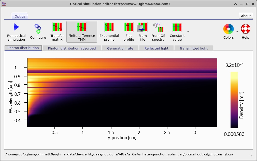
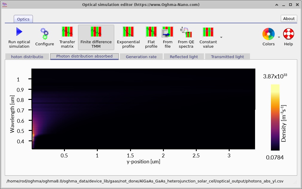
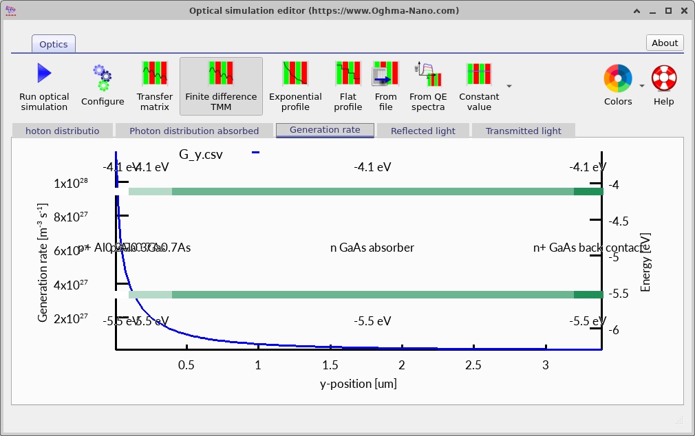
The transfer-matrix method evaluates how forward- and backward-propagating optical waves interact with a stack of layers having complex refractive indices \(\tilde n(\lambda)=n(\lambda)+ik(\lambda)\). Its field solution can account for reflection and interference; local absorption is then translated into a generation rate using photon energy. For the GaAs absorber, the wavelength-dependent absorption coefficient is an essential input because it determines where photons of different energies are absorbed inside the 2.8 µm layer.
Take particular care when interpreting the AlGaAs optical data. The electrical material model uses an explicitly specified alloy fraction, while the selected optical material database is referenced independently. Before using the calculation for quantitative spectral design, verify that the Inorganic/AlGaAs/Adachi dataset actually supplies the appropriate composition dependence at the relevant wavelengths. An electrical alloy fraction of 0.30 does not prove that every optical constant varies correctly with composition.
Similarly, the simulated 1D structure idealises the optical geometry. It does not independently model a fabricated front-metal grid, lateral current spreading, surface texture, detailed anti-reflection coatings, or defects introduced by a real epitaxial process unless those features are specifically included in the optical and electrical models. The optical analysis is thus especially useful for understanding trends and identifying likely spectral losses, while comparison to measured cells requires a carefully matched structure and calibrated material data.
12. Assumptions, checks and limitations
This example should be regarded as a working numerical demonstration of an AlGaAs/GaAs heterojunction, not a validated prediction of a particular manufactured solar cell's certified efficiency. The four-layer structure, contacts and meshing come from the supplied simulation configuration, and the screenshots show that several calculations and output views have been prepared. A reliable quantitative prediction additionally requires independently verified materials, optics, recombination coefficients, contact quality and numerical convergence.
Geometry and dimensionality. The 3D viewer is a visual rendering; the electrical and optical depth dependence in this tutorial is one-dimensional. Effects such as front-grid shading, edge losses, lateral voltage drop and nonuniform contacts are outside this baseline 1D description.
Material-model consistency. Bandgap and electron affinity in a composition-dependent alloy should come from consistent models. The electrical Lua scripts and optical \(n,k\) datasets are distinct inputs. Any override applied to only one side can unintentionally create artificial discontinuities, especially at the heterointerface.
Recombination and interfaces. Bulk SRH settings are present, but that does not prove that a real AlGaAs/GaAs interface has been represented with an experimentally validated interface-recombination velocity. Real interface quality can govern the measured voltage and carrier collection. Changes to traps and radiative/Auger processes should be tested one at a time and examined through the rate profiles.
Numerical reproducibility. Check terminal convergence for the entire J–V and intensity sweep, perform mesh refinement near the heterointerface, and test whether key photovoltaic metrics and internal profiles are stable. Failure of a particular high-intensity point is not evidence of a physical device effect. Use an unchanged baseline to distinguish physical trends from solver sensitivity.
Interpreting screenshots. Each snapshot is a state selected from the saved simulation output, and the figure numbers in this tutorial identify the screenshot index, not a guaranteed applied voltage. Read the actual voltage annotation in the OghmaNano plot before attaching a numeric voltage to a particular profile. Avoid inferring a numerical \(V_{OC}\), \(J_{SC}\), fill factor or efficiency from a small image thumbnail when the output data file provides the accurate values.