Databases
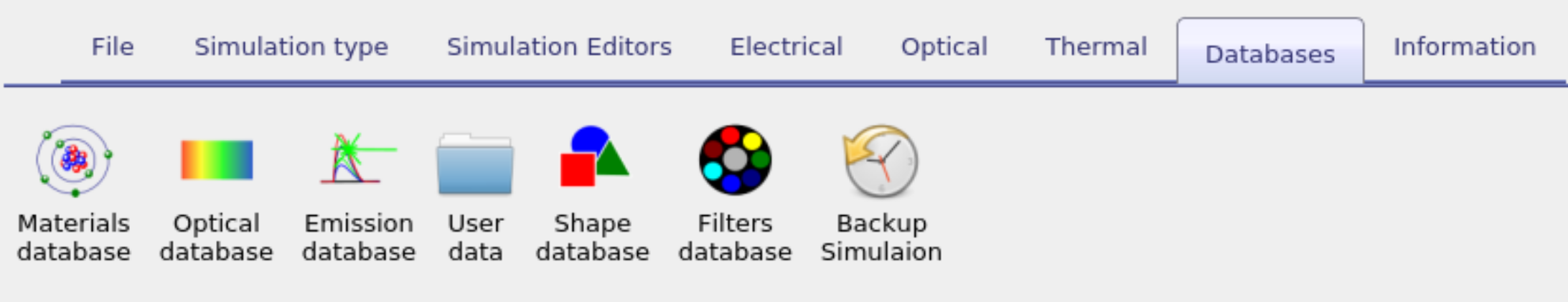
There are a series of databases used to define material parameters, shapes and solar spectra etc... These are described within this section. From the graphical user interface they can be accessed from the database ribbon, see figure 15.1.
There are two copies of these databases, one copy in the install directory of OghmaNano C:\(\backslash\)Program Files\(\backslash\)OghmaNano\(\backslash\) and one in your home directory in a folder called oghma_local. When the model starts for the first time it copies the read only materials database from, to the oghma_local folder in your home directory. If you delete the copy of the materials database in the oghma_local folder it will get copied back next time you start the model, this way you can always revert to the original databases if you damage the copy in oghma_local.
The structure of the databases are simple, they are a series of directories with one directory dedicated to each material or spectra etc.. E.g. there will be one directory called Ag in the optical database which defines silver, and another directory in the spectra database called am1.5g which defines the solar spectrum. Within each directory there is a data.json file which defines basic material properties of the material such as what it is and what icon to use for it. There may be a couple of .bib files that contain reference information for the object in bibtex format. The rest of the key information will be stored in human readable .csv files. These files can be opend in notepad or any text editor. The one exception is that in the shape database some large files are stored in a binary format.
Materials database
Related YouTube videos:
 |
A tutorial on adding new materials to OghmaNano |
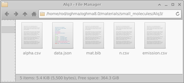
This database primarily contains n/k data and PL emission spectra. However it also contains some electrical information and some thermal information. Each subdirectory within the materials database identifies the material name. In each sub directory there are two key files \(alpha.csv\) and \(n.csv\), these files are standard text files can be opened with any text editor such as wordpad. Alpha.csv contains the absorption coefficient of the material while n.csv contains the the refractive index. The first column of the file contains the wavelength in \(m\) (not \(cm\) or \(nm\)), and the second column of the file contains the absorption coefficient in \(m^{-1}\) (for alpha.csv) and the real part of the refractive index (i.e. n) in au (for n.csv). The data.json defines the material color and any known electrical or thermal data. If the material is used in emissive optical simulations the emission spectra of the material will be stored in a file called \(emission.csv\). An example material directory, in this case Alq3 can be seen in figure 15.2, a description of these files can be found in 15.1.
| File name | Description | |
|---|---|---|
| data.json | json file infomration about the material (LUMO/HOMO levels etc..) | |
| alpha.csv | wavelength (m) v.s. absorption (\(m^{-1}\)) | |
| n.csv | wavelength (m) v.s. refractive index (au) | |
| \(emission.csv^{*see below}\) | wavelength (m) v.s. PL emission (au) | |
| mat.bib | Bibtex file containing references |
Adding new materials - the hard way
If you wish to add materials to the database which do not come as standard with the model you can do it in the following way: Simply copy an existing material directory (say oghma_local\(\backslash\)materials\(\backslash\)oxieds\(\backslash\)ito) to a new directory (say oghma_local\(\backslash\)materials\(\backslash\)oxieds\(\backslash\)mynewmaterial). Then replace alpha.csv and n.csv with your data for the new material. You can ignore the data.json file, although if you know the energy levels you can add the values in the file.
If you don’t have data to hand for your material, but you do have a paper containing the data, you use the program Engauge Digitizer, written by Mark Mitchell https://github.com/markummitchell/engauge-digitizer to export data from publications. After you have finished updating the new material directory, whenever a new simulation is generated the new material files will automatically be copied into the active simulation directory ready for use.
Adding new materials - the easy way
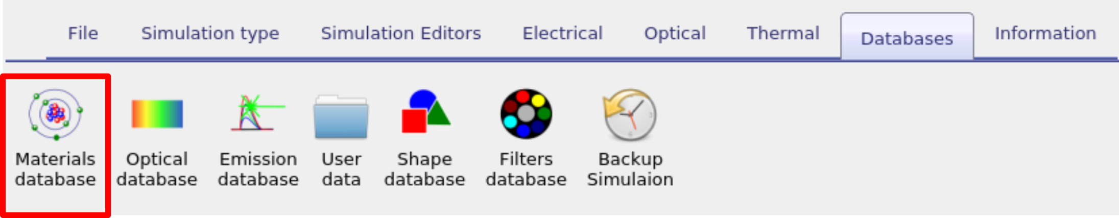
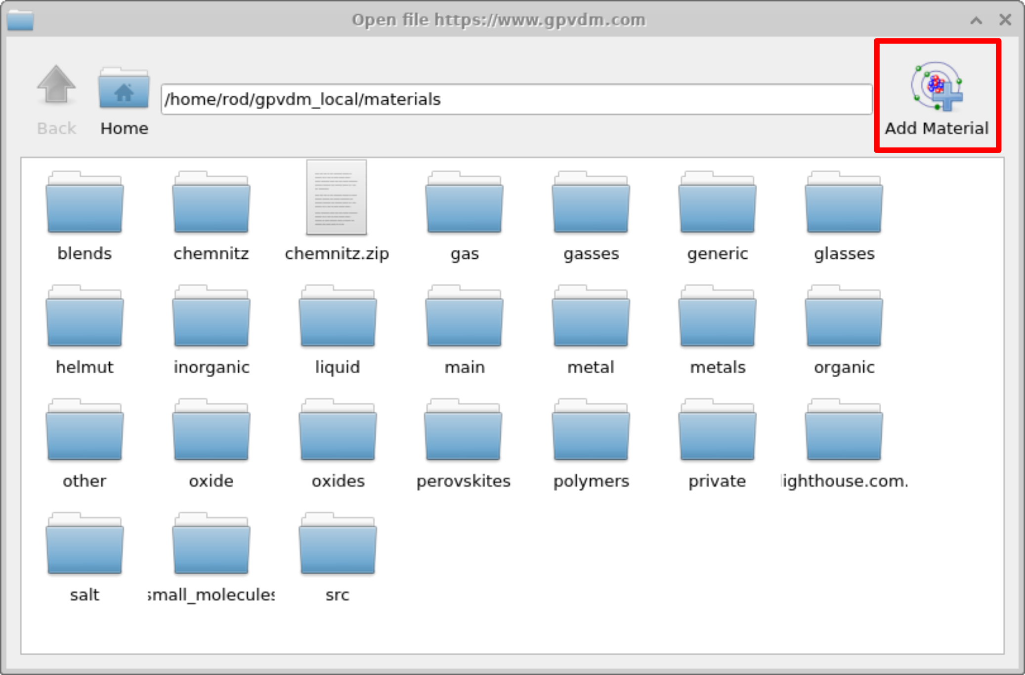
To add a new material go to the database ribbon and click on Materials database as shown in figure 15.3.
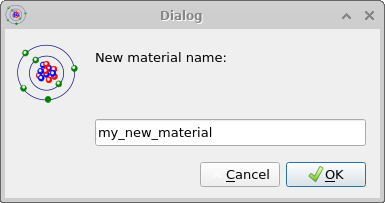
Then click add material in the top right of the window, this will bring up a dialogue box which will ask you to give a name for your new material, this is visible in figure [fig:materialadd3]. In this case we called the material my_new_material.
 [fig:materialadd2]
 [fig:materialadd3]
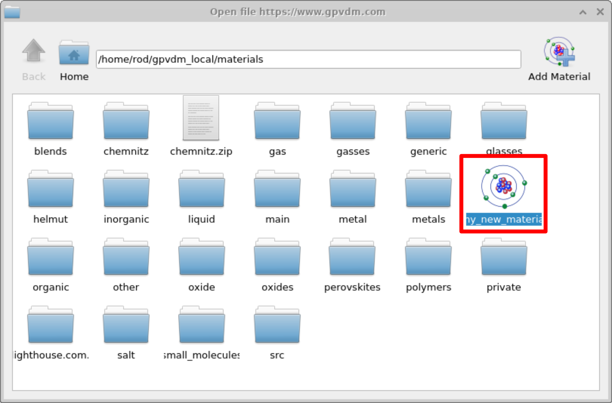
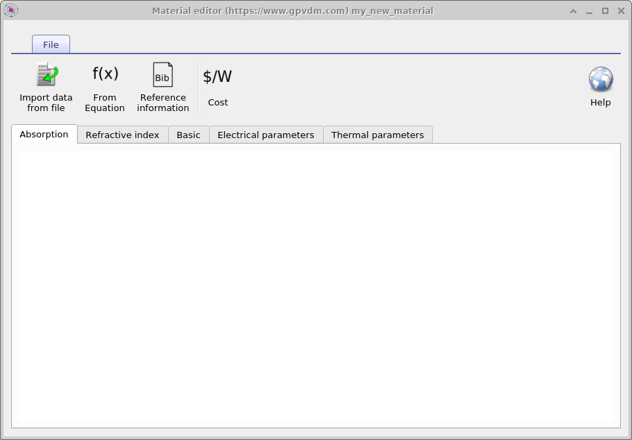
Once you have clicked OK the new material will appear see Figure [fig:materialadd4], open it by double clicking on it. This will bring up an empty material window with no data. See Figure [fig:materialadd5].
 [fig:materialadd4]
 [fig:materialadd5]
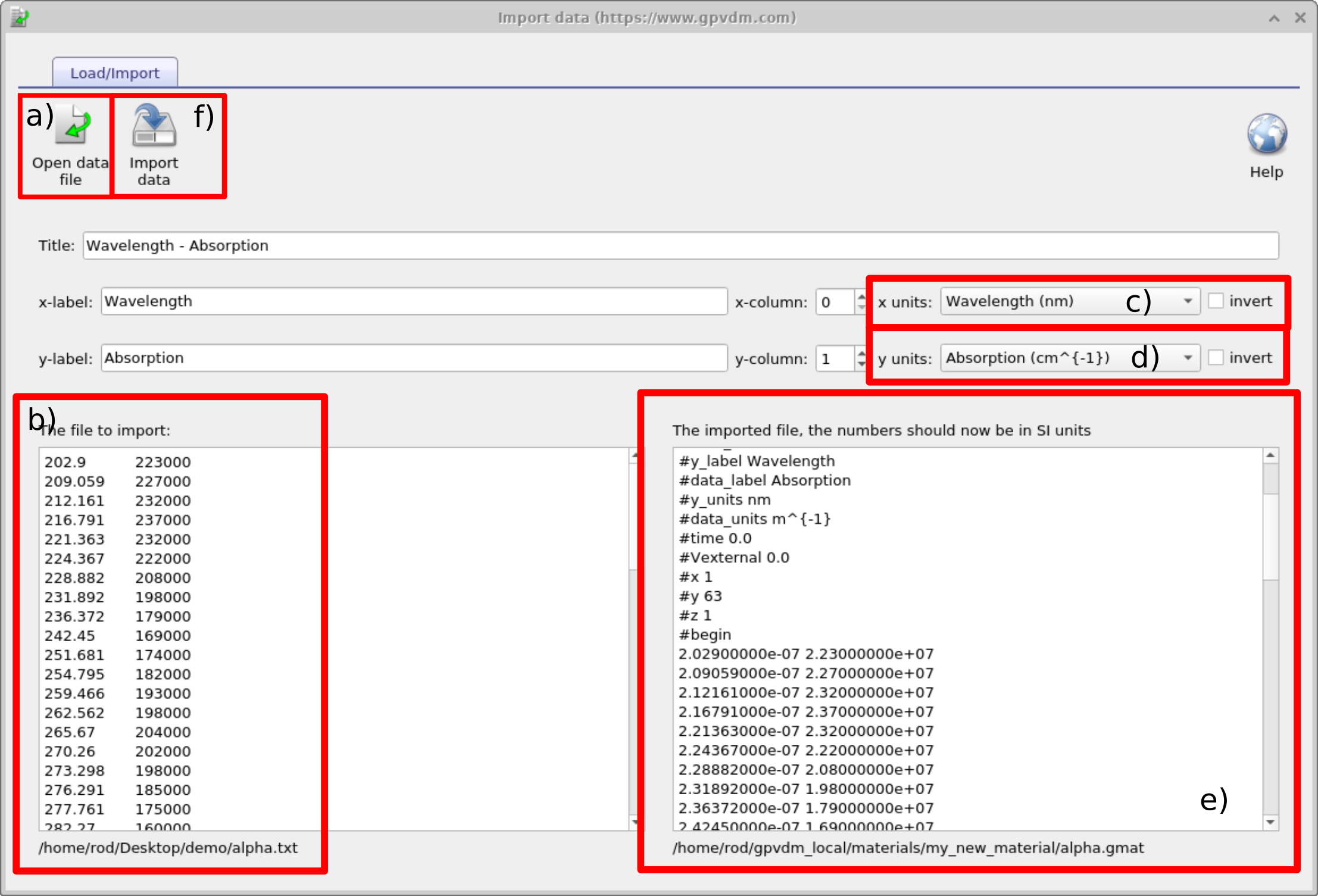
To import data to the material use the Import data from file button situated on the top left of the material window see Figure [fig:materialadd5] this will bring up the import data wizard which is shown in Figure 15.4. To use this wizard follow these steps:
-
Open a file you want to import. The file can only be a text file or a csv file.
-
Once the file has been loaded it will be visible in the text box on the left.
-
Select the units of the x-axis of the original file.
-
Select the units of the y-axis of the original file.
-
The file should appear converted into SI units on the right hand text box.
-
If you have happy with the conversion click import data and the data will be saved.
This process can be seen in 15.4, once done the imported data will appear in the material as shown on the top left of 15.8. In this example absorption data was imported, for the material to be used in a simulation the refractive index (real part) will also need to be imported.
 |
 |
 |
 |
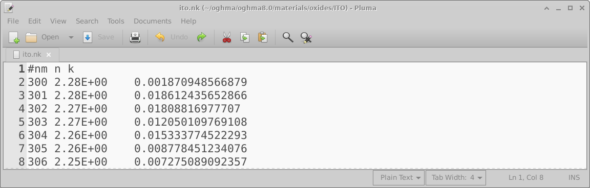
But I have a data in nm/n/k format
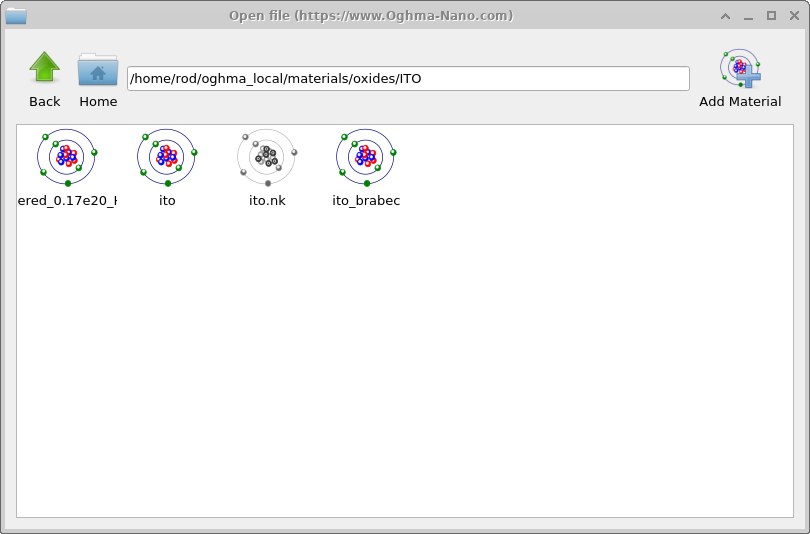
Usually OghamNano only accepts data input in SI units and usually only accepts input in one format. This is to reduce the overall number of lines of code and reduce maintenance. However, I have been asked to make the model accept data of format: wavelength (nm), refractive index (au), k (au), as shown in Figure 15.9. OghmaNano will be able to read this file if you simply copy it into your_home_directory\(\backslash\)oghma_local\(\backslash\)materials and give it a file extension .nk, so for example ito.nk. Where your_home_directory is simply your Windows home directory. It is usually located on the C:\(\backslash\)Users on a home PC but the location can change if you are on a corporate PC. Once you have dragged the file into your_home_directory\(\backslash\)oghma_local\(\backslash\)materials it will appear as a material in the model. See Figure 15.10. You can see that the .nk file in Figure 15.10 is greyed out, this is because it is a non standard OghamNano file, that OghmaNano can read but not edit.
Shape database
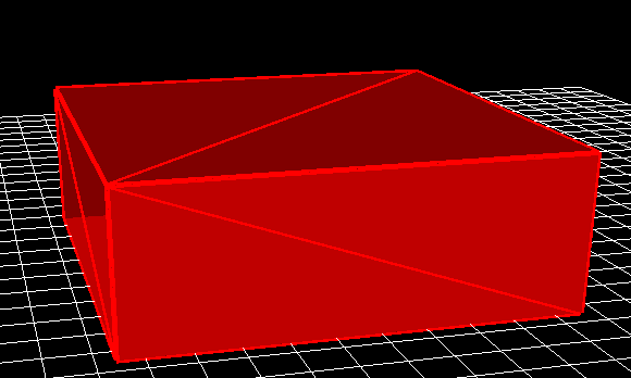
All physical objects within a simulation are shapes. For example the following things are all shapes; a layer of a solar cell; a layer of an OLED; a lens; a complex photonic crystal structure; contact stripe on an OFET; the complex hexagonal contact on a large area device (see figure 1.1 for more examples). These shapes are defined using triangular meshes for example a box which is used to define layers of solar cells, and layers of LEDs is defined using 12 triangles, two for each side. This box structure can be seen in figure 15.11.
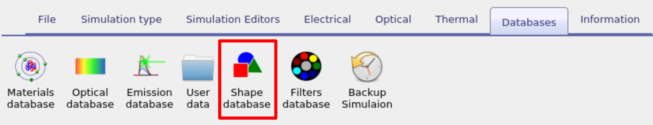
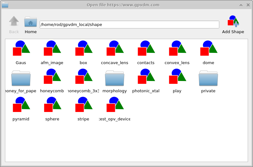
Shapes are stored in the shape database, this can be accessed via the database ribbon and clicking on the Shapes icon, see figure 15.12. By clicking on the shape database icon the shape database window can be brought up see figure 15.13.
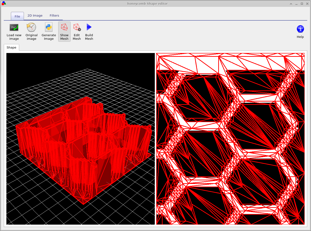
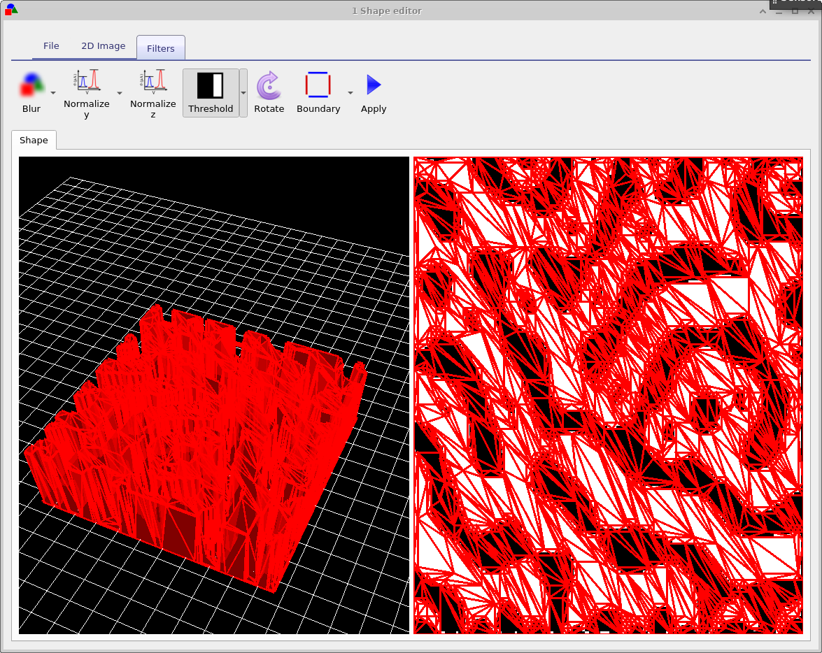
Try opening some of the shapes and have a look at them. You will get a window much like that shown in figure 15.14. Figure 15.14 shows a honeycomb contact structure of a solar cell. On the left of the window is the 3D shape, and on the right of the window is the 2D image which was used to generate it. Overlaid on the 2D image is a zx projection of the 3D mesh. The process of generating a shape involves first defining a 2D png image which you want to turn into a shape, in this case the 2D image is a series of hexagons and a bar at the top. This image is then converted into a triangular mesh using a discretization algorithm.
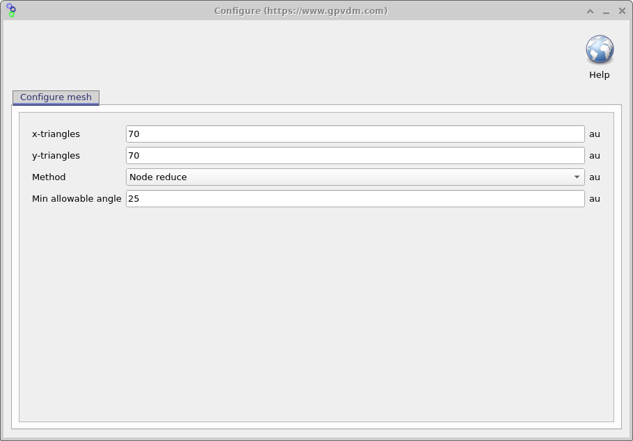
Now try opening the shape morphology/1 and you should see a window such as the one shown in figure 15.16, in the file ribbon find the icon which says show mesh. Try toggling it of and on, you will see the 2D mesh become hidden and then visible again. This example is a simulated bulk heterojunction morphology, but you can turn any 2D image into a shape by using the load new image button in the file ribbon. Try opening the mesh editor by clicking on Edit Mesh the file ribbon, you should get a window looking like figure 15.17. This configure window has three main options x-triangles, y-triangles and method. The values in x-triangles, y-triangles determine the maximum number of triangles used to discretize the image on the x and y axis. Try reducing the numbers to 40 then click on Build mesh in the file ribbon.
 |
 |
You will see that the number of triangles used to describe the image reduce. The more triangles that are used to describe the shape the more accurately the shape can be reproduced, however the more triangles are used the more memory a shape will take up and the slower simulations will run. There is always a trade off between number of triangles used to discretize a shape. Try going back to the Edit Mesh window and set method to no reduce and then click on Build mesh from the file menu again. You will see that the complex triangular mesh as been replaced by a periodic triangular mesh, which is more accurate but requires the full 70x70 triangles. The difference between the no reduce and Node reduce options are that no reduce simply uses a regular mesh to describe and object and Node reduce starts off with a regular mesh then uses a node reduction algorithm to minimize the number of triangles used in the mesh.
As well as loading images from file, the shape editor can generate it’s own images for standard objects used in science, the 2D image ribbon is visible in the right hand panel of figure 15.16. There are options to generate lenses, honeycomb structures and photonic crystals. Each button has a drop down menu to the right of it which can be used to configure exactly what shape is generated.
The final ribbon to be discussed is the Filters ribbon. This is used to change loaded images, try turning on and off the threshold function. This applies a threshold to an image so that RGB values above a given value are set to white and those below are set to black. There are also other functions such as Blur, and Boundary which can be used to blur and image and apply boundaries to an image.
The shape file format
A shape has to be a fully enclosed volume, if you use the built in shape discretizer this will be done for you automaticity. However if you are building shapes by hand you will have to enforce this condition. Each shape directory contains the following files
| File name | Description | |
|---|---|---|
| \(data.json\) | Holds the configuration for the shape file | |
| \(image\_original.png\) | backup of the imported image | |
| \(image\_out.png\) | The final processed image | |
| \(image.png\) | The imported image which may be modified. | |
| \(shape.inp\) | The discretized 3D structure. |
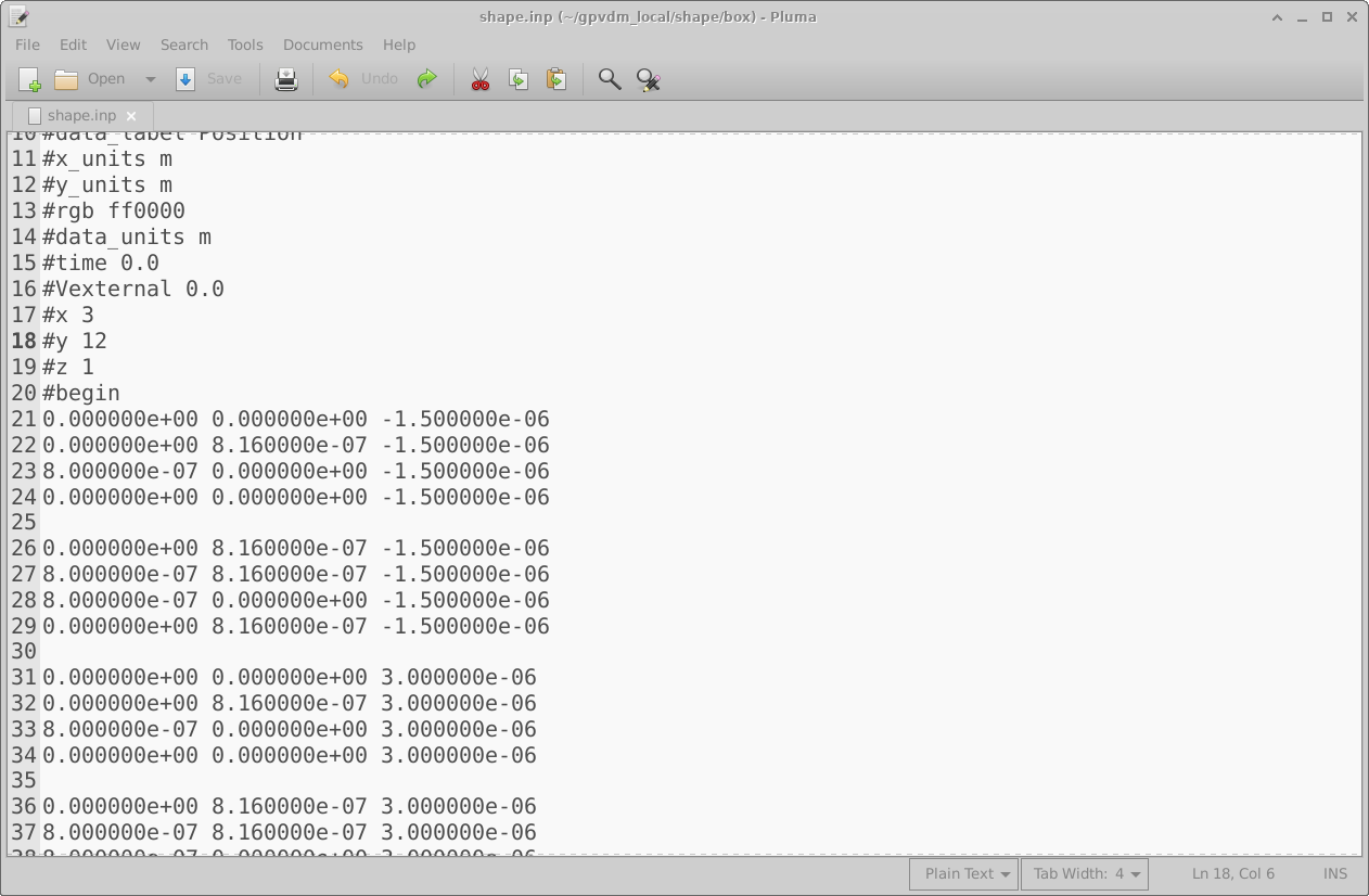
The png files are of images in various states of modification. The data.json file stores the configuration of the shape editor and the shape.inp file contains the 3D structure of the object. An example of a shape.inp file is shown below in 15.19. The file format has been written so that gnuplot can open it using the splot command without any modification. As such each triangle is comprised of four z,x,y points (lines 21-24), the first three lines define the triangle, and the forth line is a repeat of the first line so that gnuplot can plot the triangle nicely. The number of triangles in the file is defined on line 18 using the #y command. The exact magnitudes of the z,x,y values do not matter because as soon as the shape is loaded all values are normalized so that the minimum point of the shape sits at 0,0,0 and the maximum point from the origin sits at 1,1,1. When being inserted into a scene, the shape is then again renormalized to the desired size of the object in the device.
Filters database
This contains optical filters.
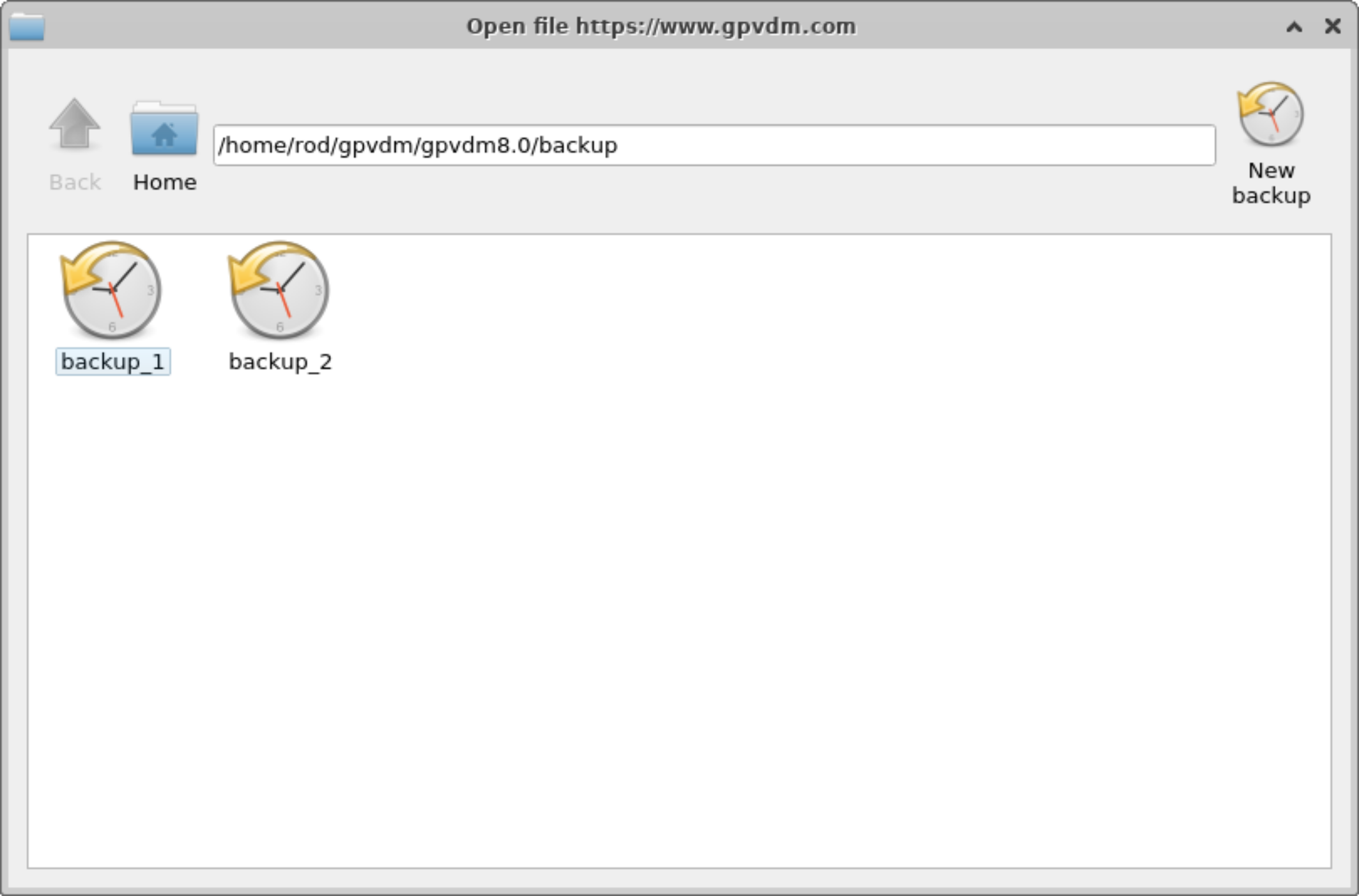
Backups of simulations
Very often when running a simulation you want to make a copy of it before continuing to play with the parameters. To do this click on the backup simulation button in the database ribbon (see figure 15.1), this will bring up the backup window, see figure 15.20. If you click on the "New backup" icon on the top right of the window, a backup will be made of your current simulation. And an icon representing the backup will appear in the backup window. To restore the backup double click on the icon representing your stored simulation. Note this backup is only stored in the your local simulation directory, and is more of a checkpoint than a real backup.... so make sure you have other copies of your simulation if it is very important to you..