

Perovskite/Silicon Tandem Solar Cell Simulation: Device Structure, Drift-Diffusion, J-V Curves and Optical Generation
1. Introduction: why combine perovskite and silicon?
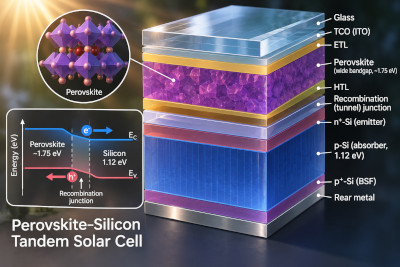
A conventional solar cell uses one semiconductor junction to convert sunlight into electricity. Its bandgap determines which photons can be absorbed. Photons with energies below the bandgap normally pass through without creating an electron-hole pair, while much of the energy of photons far above the bandgap is lost as energetic carriers relax towards the band edges. A tandem solar cell places two photovoltaic absorbers with different bandgaps along the optical path, allowing each to convert a different portion of the solar spectrum.
In a perovskite/silicon tandem, a relatively wide-bandgap perovskite top cell absorbs much of the visible light. Lower-energy photons transmitted by the top cell can then be absorbed by a narrower-bandgap crystalline-silicon bottom cell. The two cells work together: the top cell is particularly useful for harvesting high-energy photons, while the silicon cell extends the useful response into the near infrared. This spectral division is why tandems are of such interest for higher-efficiency photovoltaics.
The example used here is a monolithic two-terminal (2T) tandem. Both junctions are incorporated in a single multilayer structure, with one external front contact and one rear contact. The subcells therefore operate electrically in series: they share a common terminal current, while their generated voltages contribute to the total device voltage. An internal recombination connection lets the carrier currents pass from one photovoltaic junction to the next.
This tutorial walks through a supplied OghmaNano simulation, examines the semiconductor and optical settings, runs the illuminated J-V calculation, and interprets the saved results. Rather than building every layer from scratch, we will use the example to explore how optical absorption, carrier transport, junction electrostatics and recombination combine to determine tandem behaviour.
2. Opening the tandem solar-cell example
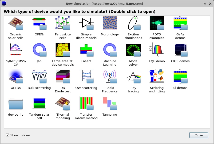
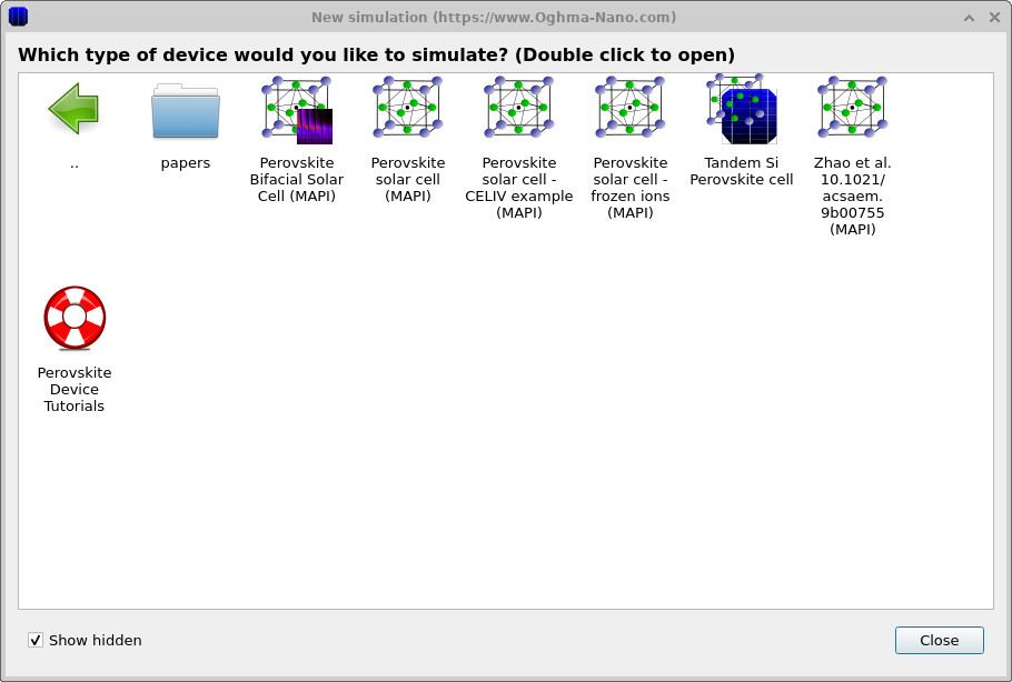
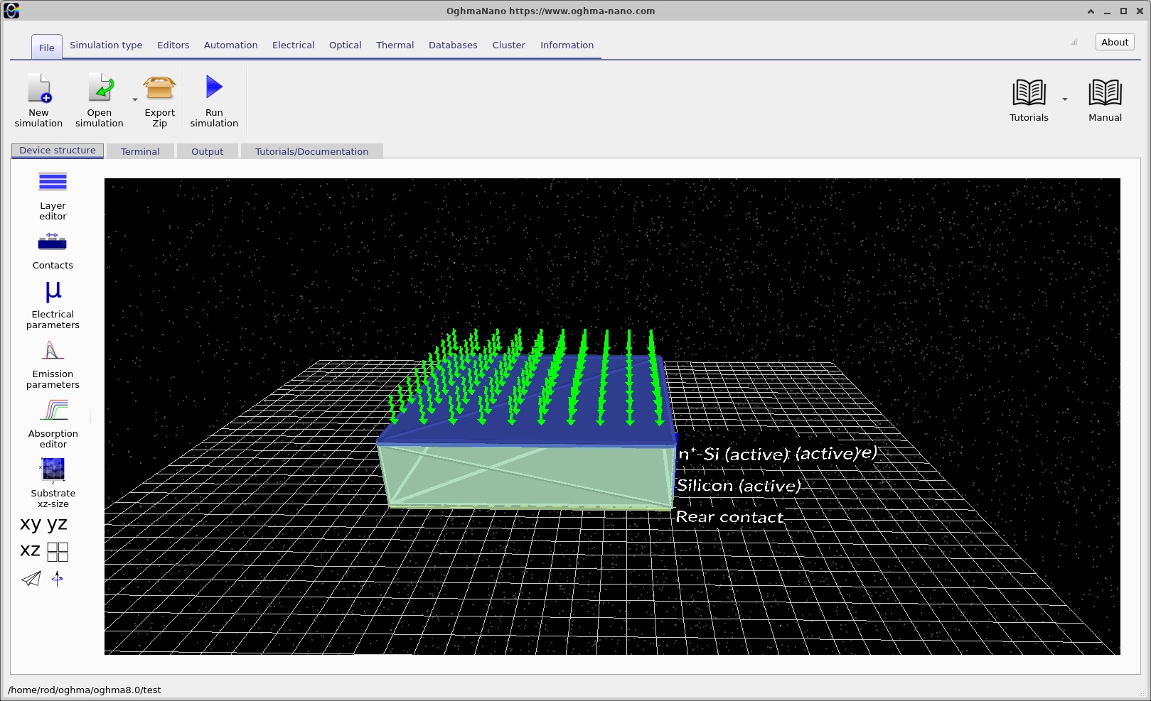
Start OghmaNano and choose New simulation. The example browser is shown in ??. Navigate to the collection containing the perovskite/silicon tandem example and open it; ?? shows a subsequent view of the example selection. When the simulation loads, the Device structure tab displays the stacked device (??).
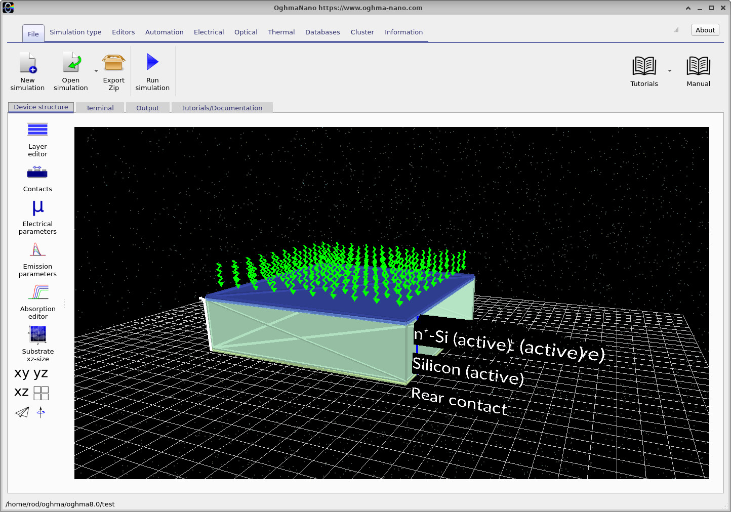
Take a moment to identify the Device structure, Terminal and Output areas of the main window. The first is where you inspect the layer stack and its settings. The Terminal shows the progress of numerical calculations, while Output contains the generated data files and plots. Save a working copy of the example before making modifications so that you can easily return to the original configuration.
3. The perovskite/silicon layer stack
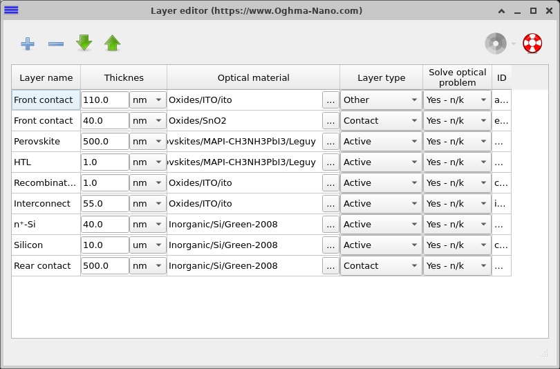
Open the Layer editor (??). The example contains nine listed regions, including optical/contact layers and the semiconductor regions used in the electrical calculation. The most useful way to understand the stack is to read it from the illuminated front surface towards the aluminium-side rear contact.
| Layer (front to rear) | Thickness | Purpose |
|---|---|---|
| ITO front contact | 110 nm | Transparent conducting front electrode in the optical stack. |
| SnO2 front transport/contact region | 40 nm | Electron-selective transport region on the perovskite side. |
| Perovskite | 500 nm | Wide-bandgap top photovoltaic absorber (electrical bandgap 1.63 eV). |
| HTL | 1 nm | Effective hole-selective layer at the back of the perovskite. |
| Recombination | 1 nm | Effective carrier recombination junction between the two subcells. |
| ITO interconnect | 55 nm | Conducting intermediate layer linking the photovoltaic regions. |
| n+-Si | 40 nm | Donor-doped silicon emitter. |
| Silicon | 10 µm | Acceptor-doped crystalline-silicon bottom absorber (bandgap 1.12 eV). |
| Rear contact | 500 nm | Rear optical/contact region; the supplied JSON uses a silicon optical dataset in this region. |
The structure contains two fundamentally different light absorbers. The 500 nm perovskite is thin, with a larger bandgap, whereas the 10 µm silicon is thicker and absorbs lower-energy photons. The perovskite and silicon are not simply connected by placing their absorbers in contact: the HTL, recombination region, ITO interconnect and doped silicon emitter together establish the electrical connection between them.
The ITO at the front and the ITO within the device have different jobs. Front ITO provides a transparent electrode; buried ITO provides a conducting interconnection between subcells. It is therefore entirely reasonable for ITO to appear twice in one tandem stack. The screenshot of the layer editor is useful for checking the material assignments and thicknesses before changing anything.
4. Doping profiles and electrical material parameters
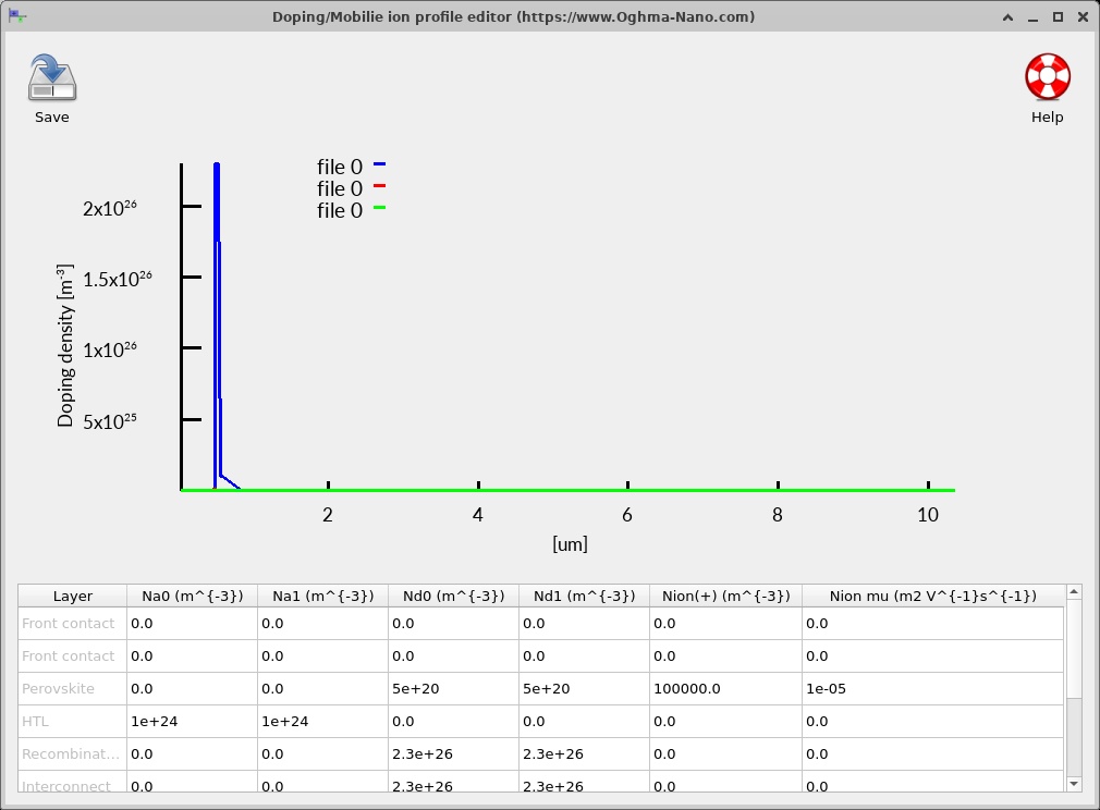
Choose Doping / Ions to inspect the doping distribution (??). The silicon part contains a highly donor-doped n+ emitter adjacent to a more lightly acceptor-doped p-type absorber. These form the silicon photovoltaic junction. The upper perovskite stack instead relies on its transport-layer contacts and electronic band alignment to select electrons and holes.
In a semiconductor, ionised dopants contribute to the space charge in Poisson’s equation. The resulting internal electric field influences carrier collection and the spatial bending of the conduction and valence bands. Doping also changes majority- and minority-carrier populations and can therefore influence recombination. It is worth comparing the doping view with the band and carrier-density plots later in this tutorial: one shows the fixed ionised background, while the others show the self-consistent response of the mobile carriers.
The example uses a silicon emitter donor density of approximately 1025 m−3 and a silicon absorber acceptor density of approximately 1.8 × 10²² m−3. OghmaNano stores these values in SI units; to convert concentrations from m−3 to cm−3, divide by 106.
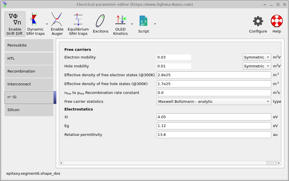
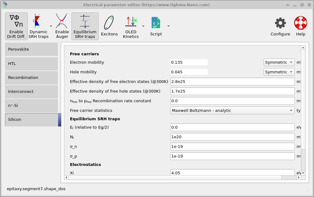
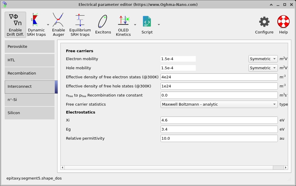
Open the Electrical parameter editor and select the n+-Si and Silicon tabs. The two panels (?? and ??) contain the electrical properties assigned to the emitter and absorber, including bandgap, effective densities of states, mobility and recombination options. In the supplied model both silicon regions have an electrical bandgap of 1.12 eV and electron affinity of 4.05 eV. Their identical material band edges and differing doping allow the built-in field to develop at the silicon p-n junction.
The silicon absorber is configured with higher bulk mobilities than the heavily doped emitter. Its electron mobility is approximately 0.135 m2 V−1 s−1 and its hole mobility approximately 0.045 m2 V−1 s−1. The perovskite uses a 1.63 eV electrical gap, with electron and hole mobilities of approximately 0.0035 m2 V−1 s−1. These parameters are relevant to how carriers traverse each absorber under illumination and applied voltage.
OghmaNano solves Poisson's equation together with the electron and hole continuity equations to calculate charge transport through the tandem solar cell. In the drift-diffusion approximation, the electron and hole current densities are given by
\[ J_n = q\mu_n n\frac{\partial E_c}{\partial y} + qD_n\frac{\partial n}{\partial y}, \qquad J_p = q\mu_p p\frac{\partial E_v}{\partial y} - qD_p\frac{\partial p}{\partial y}. \]Here, \(n\) and \(p\) are the free electron and hole densities, \(\mu_n\) and \(\mu_p\) are their mobilities, \(D_n\) and \(D_p\) are the diffusion coefficients, and \(E_c\) and \(E_v\) are the conduction- and valence-band energies expressed in eV. The band-edge gradients describe the driving forces for carrier transport, including the effects of electrostatic potential and material properties.
The equations are solved self-consistently with carrier generation and recombination. This is particularly important in a tandem device, where changes in bandgap and electron affinity influence carrier transport across multiple semiconductor interfaces. For a detailed derivation, see the OghmaNano drift-diffusion theory and the semiconductor interface theory.
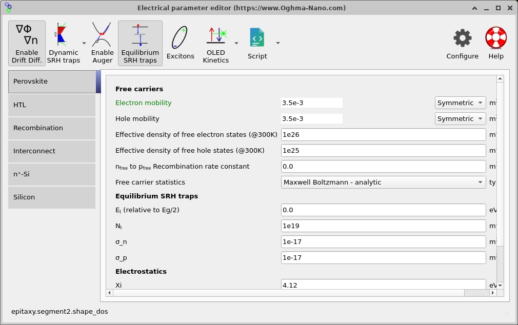
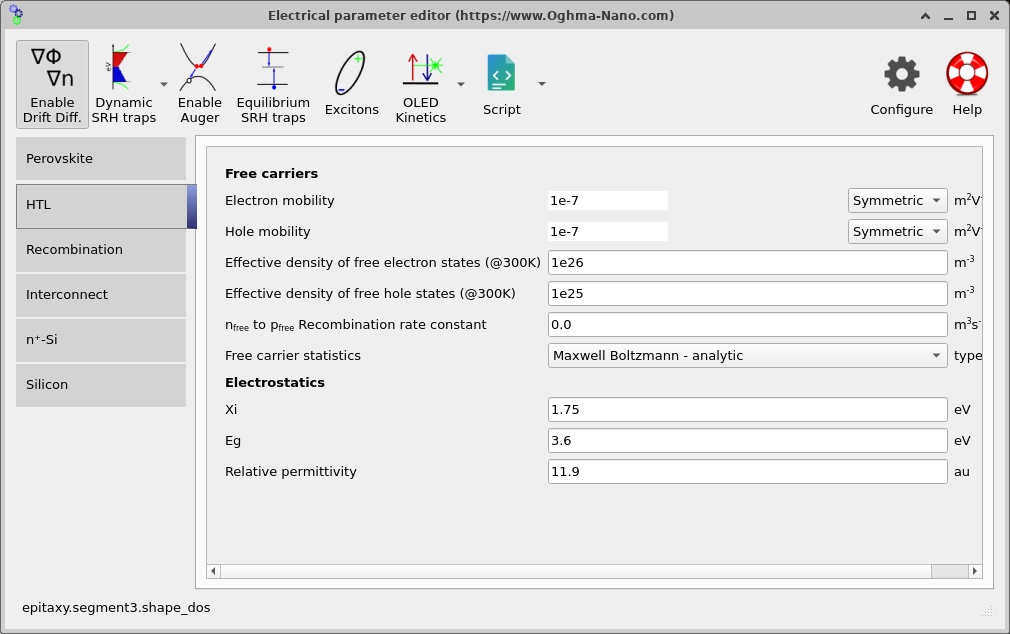
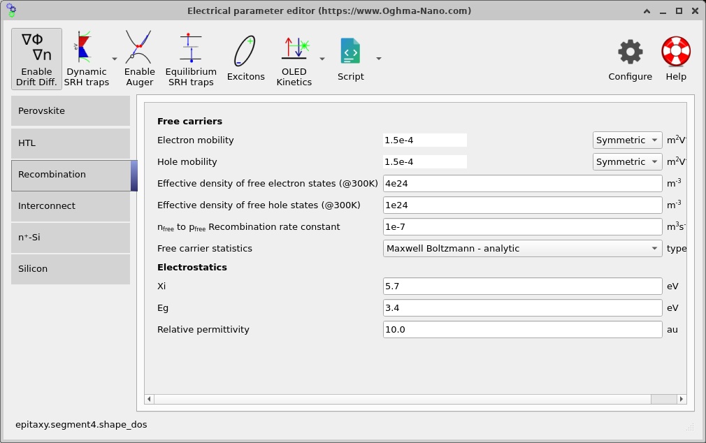
5. Connecting the two photovoltaic junctions
The most distinctive feature of a two-terminal tandem is its internal electrical interconnection. The top and bottom photovoltaic junctions are in series, so the current delivered through the complete device must be the same through both. The voltages established by the subcells can add together, provided that the connection between them does not introduce excessive loss.
The model includes an effective 1 nm recombination region and a 55 nm ITO interconnect. In this example, the recombination region uses a deliberately strong free-electron-to-free-hole recombination channel. It provides a practical way to represent the internal annihilation of opposite carriers at the series connection, where charge from the upper and lower photovoltaic junctions meets.
\[R_{\mathrm{rec}}=B\left(np-n_i^2\right).\]The example uses an effective coefficient B = 10−7 m3 s−1 in this thin region. Its function is to make the tandem’s interconnection sufficiently recombination-active; it is an effective junction parameter, not a measured radiative coefficient for bulk ITO. The two ITO regions have separate optical positions, and the recombination-layer settings should be interpreted in the context of that electrical connection.
For a two-terminal tandem, the subcells are current matched electrically. If one subcell could deliver less photocurrent than the other under otherwise independent short-circuit conditions, the full tandem operating point adjusts so that both carry a common current. This is why changes to the top-cell absorption spectrum can affect the operation of the lower cell even when none of the silicon parameters have been modified.
6. Contacts, interface settings and numerical mesh
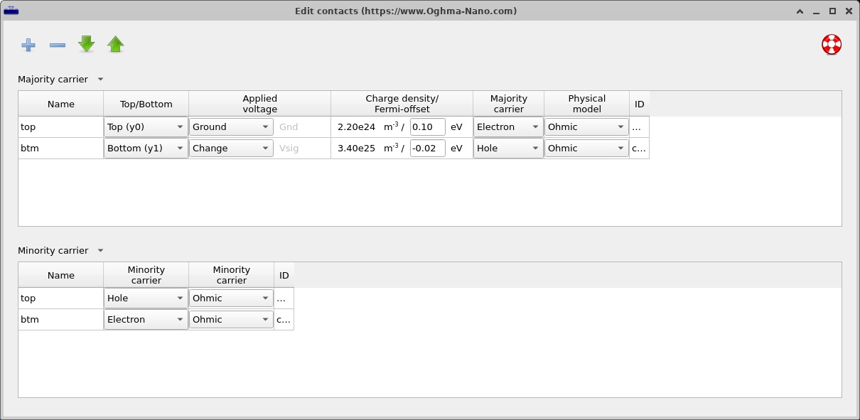
Open the Contacts editor (??) to inspect the top and bottom electrical terminals. In this one-dimensional calculation, the contacts define the voltage applied across the full tandem and the boundary conditions for carrier extraction. They should not be confused with the optical front-contact and rear-contact layers visible in the structure editor.
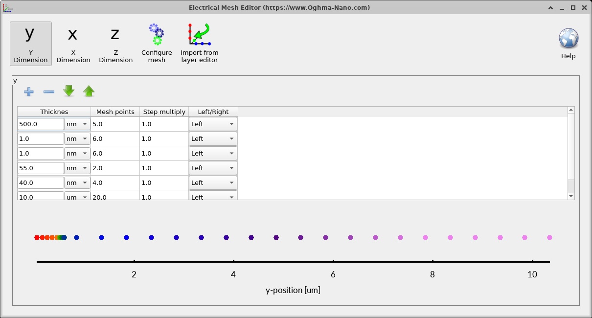
Next open the Electrical mesh editor (??). OghmaNano uses a one-dimensional y-direction electrical mesh, following the layer-normal direction. The mesh divides the perovskite, effective interconnection, silicon emitter and silicon absorber into numerical intervals over which carrier densities and electrostatic potential are calculated.
Small layers and thick absorbers impose different resolution needs. The HTL and recombination region are each about 1 nm thick, while the silicon absorber extends over 10 µm. A good mesh places sufficient points near abrupt material and doping transitions and still resolves the much larger silicon region. The supplied electrical mesh contains nominal segment counts of 5, 6, 6, 2, 4 and 20 over its six electrically modelled regions. If you later change the thickness or doping of a layer, inspect the mesh before interpreting the results.
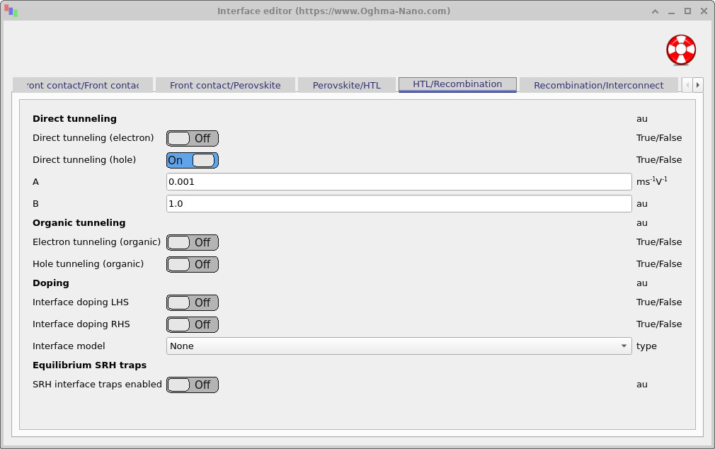
The Interface editor (??) provides the controls for interface-related transport and recombination options. For this first walkthrough, retain the supplied values. The purpose of the baseline calculation is to observe how the configured cell behaves before exploring the effects of individual interface parameters.
7. Running the illuminated current-voltage simulation
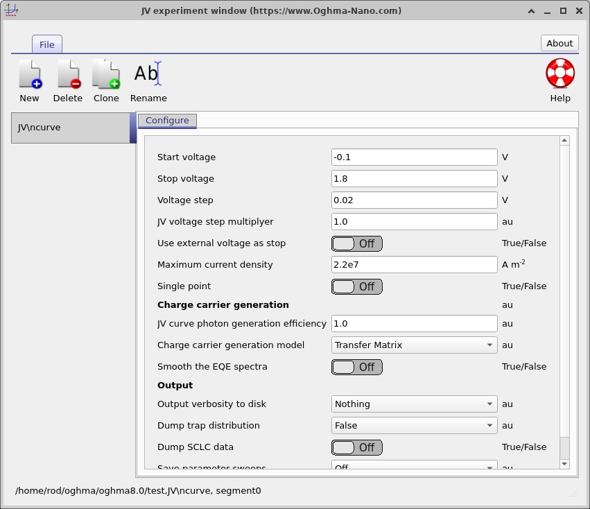
From the simulation-mode controls, choose J-V and open its editor (??). The supplied sweep starts at −0.10 V, stops at 1.80 V and uses 0.02 V steps. The illumination source uses the AM1.5G solar spectrum with a one-sun intensity multiplier. Charge-carrier generation is calculated using the optical transfer-matrix model.
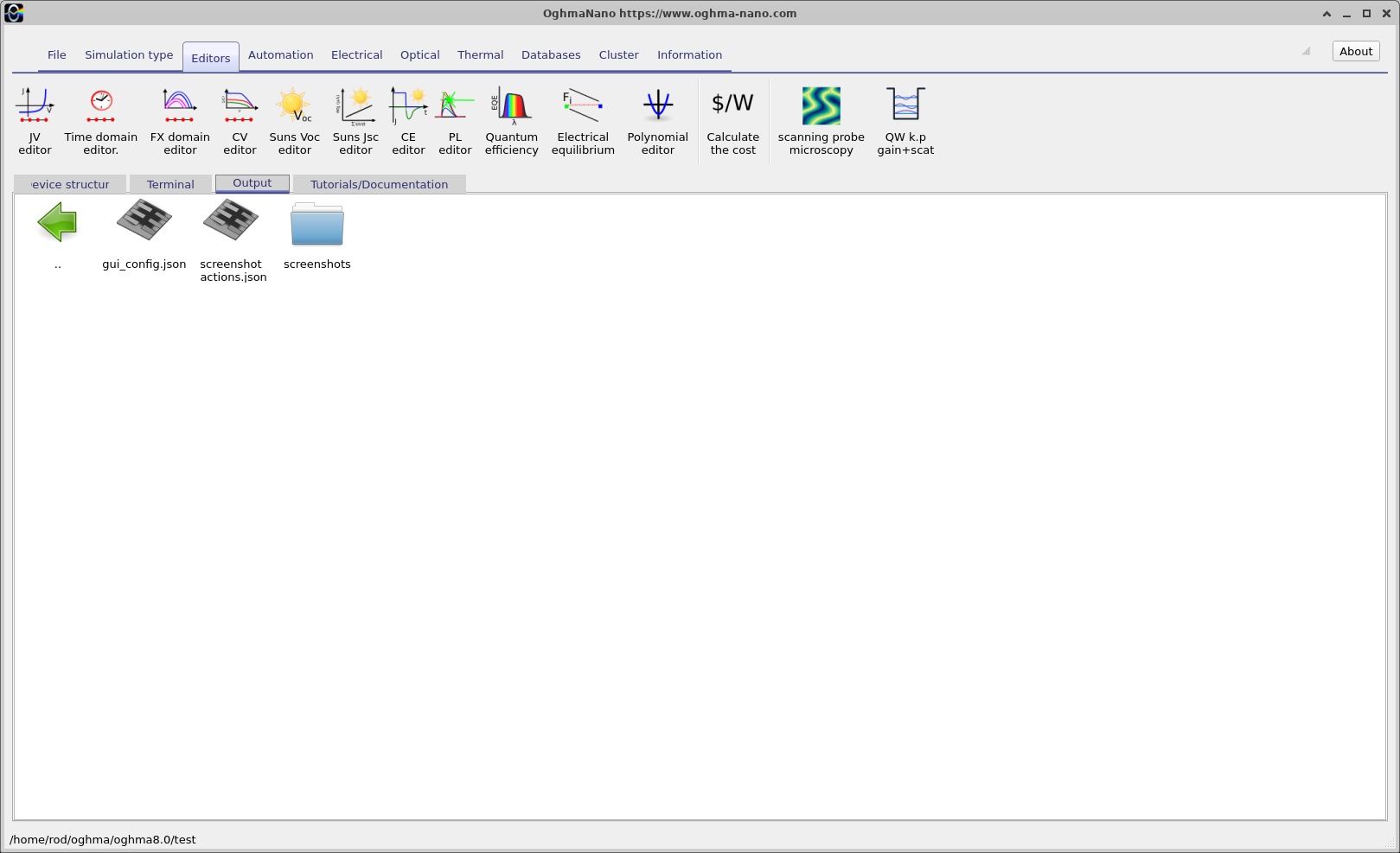
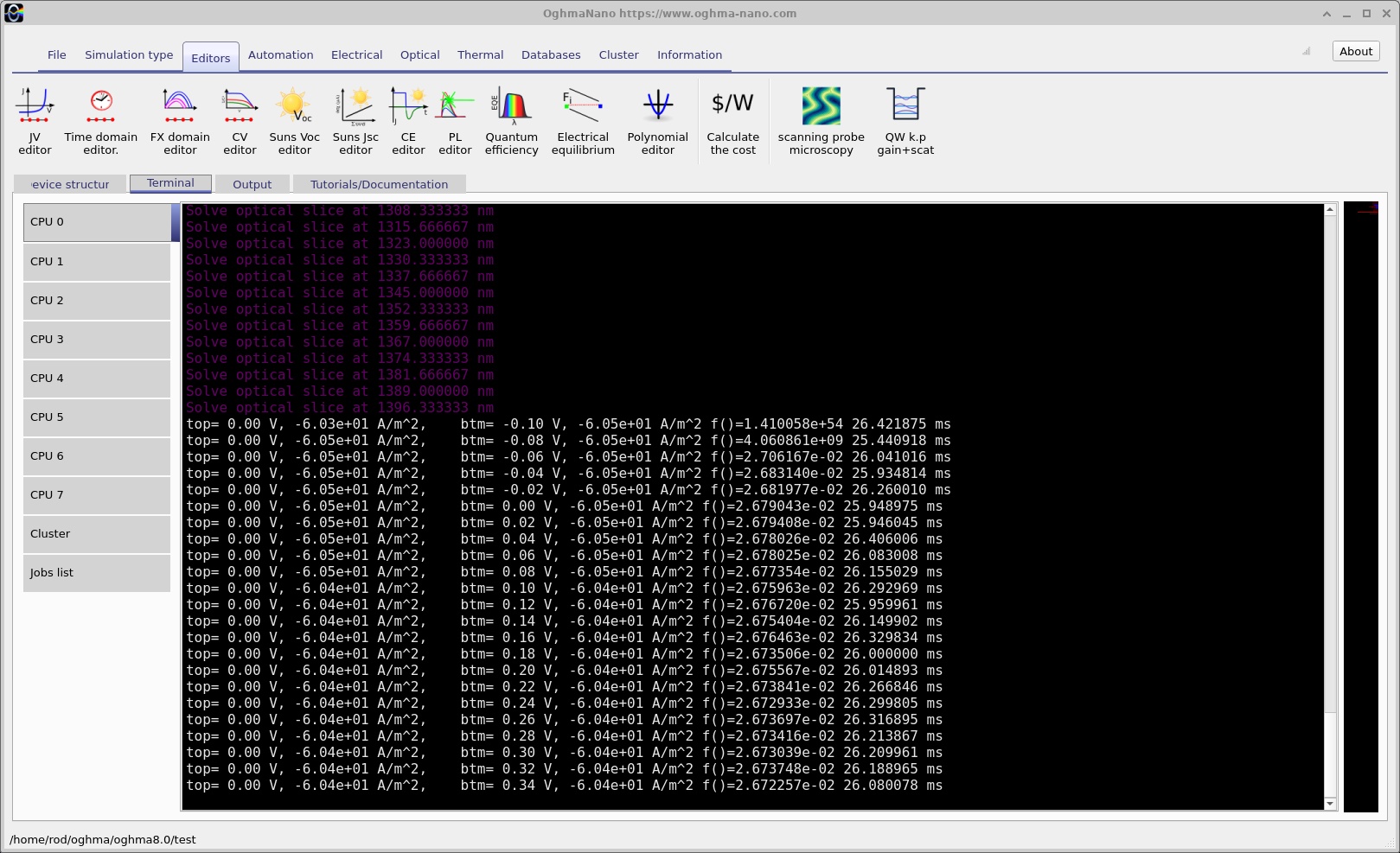
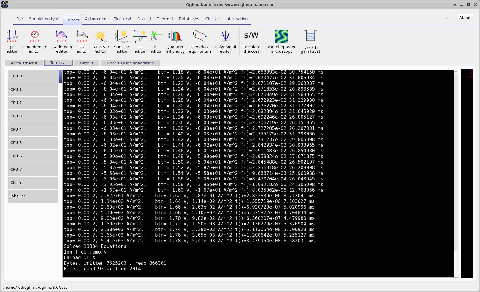
Before starting the run, inspect the Output tab (??). Click Run simulation. The Terminal tab displays the progress of the calculation; ?? and ?? illustrate two stages of the computation. When the run finishes, return to Output (??) to browse the results.
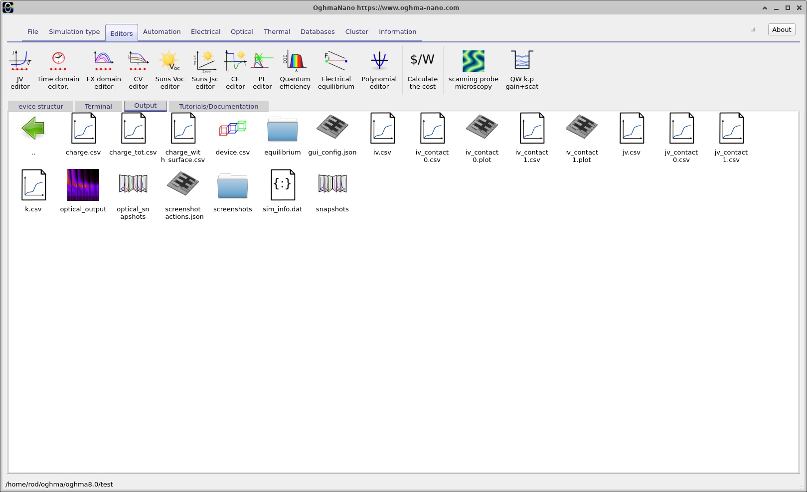
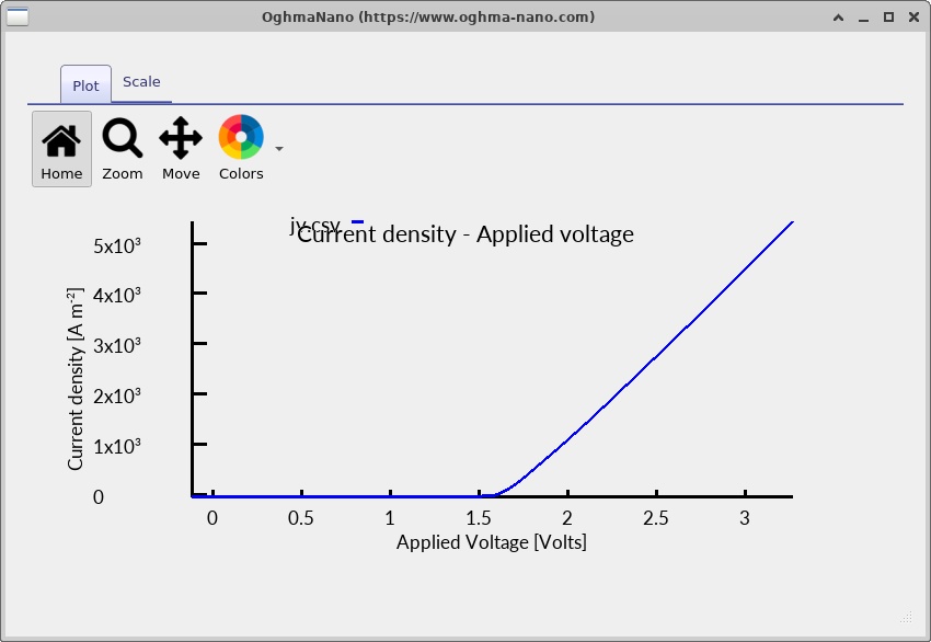
Open the saved jv.csv file to view the illuminated current-voltage curve. A solar cell has two especially useful intercepts: the short-circuit current density, measured at zero terminal voltage, and the open-circuit voltage, at which the external current density is zero. Between these operating points is a maximum-power point where the cell delivers its largest useful electrical power density.
For a tandem device it is especially useful to remember that the measured terminal current is the common current of both subcells, not the sum of two independent short-circuit currents. The tandem voltage includes the contributions from both photovoltaic junctions. This makes the tandem J-V curve a convenient overall performance indicator, while the spatially resolved plots reveal how that performance is produced.
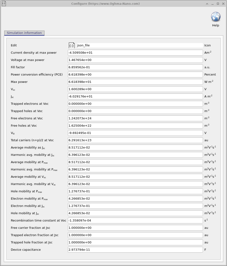
The Simulation information panel provides run and output details. Read numerical performance values from the data files or simulation-information output rather than estimating them from the thumbnail image. The screenshots guide you to the correct controls; the CSV outputs are the appropriate source for exact current, voltage and efficiency values.
8. Inspecting band structure and carrier populations
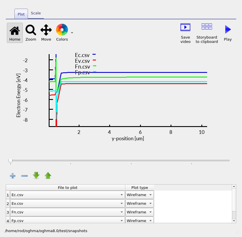
The J-V curve describes the entire device, but it does not tell us where the internal electric fields occur or how electron and hole populations change through the stack. OghmaNano can save internal profiles at different points in the voltage sweep. Open the saved band and carrier-density outputs and use the snapshot slider to move through the stored bias points.
8.1. Band diagram across both subcells
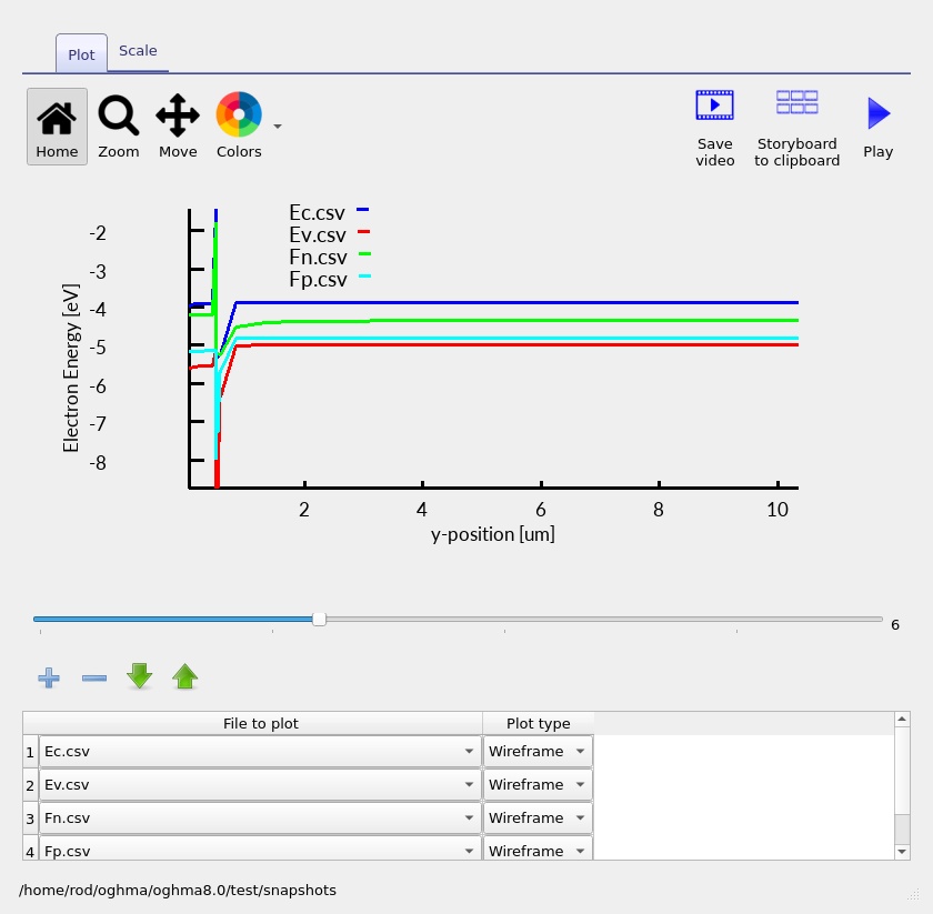
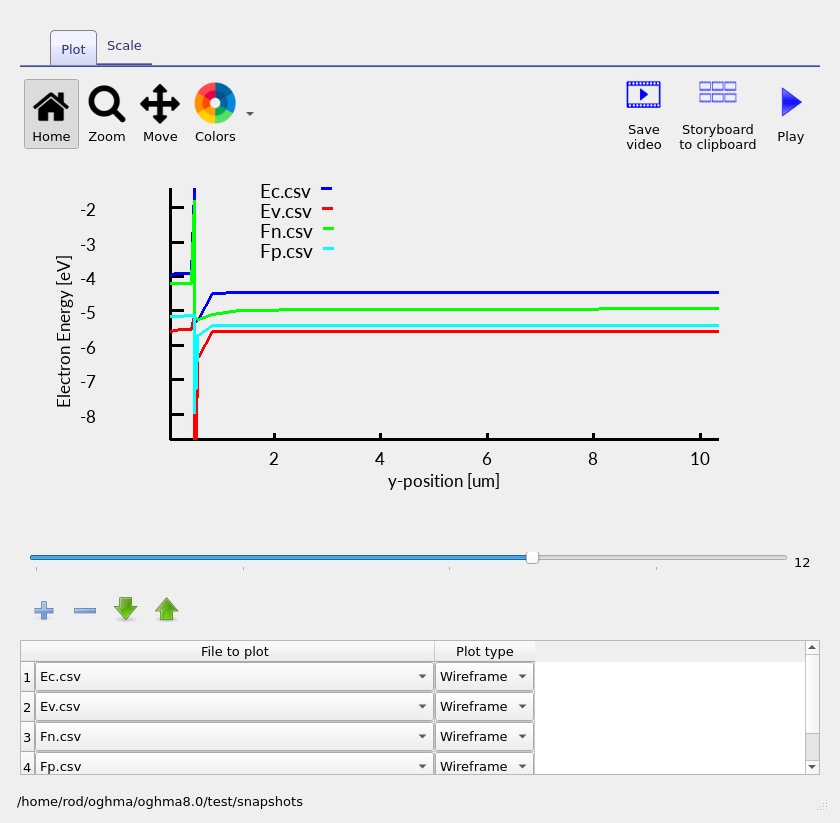
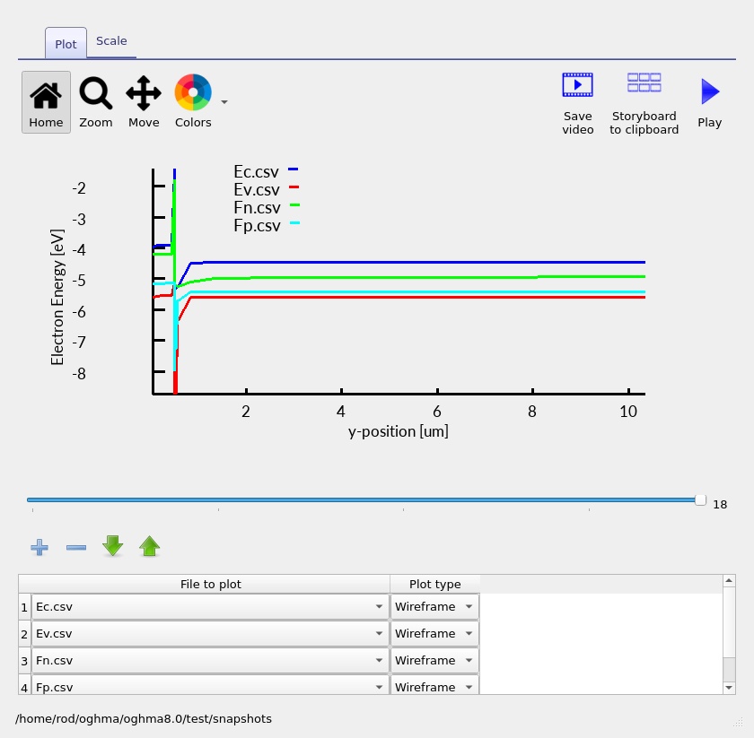
The band structure plots show how the local conduction-band edge, valence-band edge and carrier electrochemical potentials vary through the device. A change in material bandgap or electron affinity appears as a material-related band-edge change, while the smoother bending of the bands is associated with the electrostatic potential established by charge and boundary conditions.
In the perovskite region, the larger electrical bandgap helps explain why this top cell preferentially harvests higher-energy photons. In the silicon region, the smaller 1.12 eV gap permits absorption further into the near infrared. The n+/p silicon junction creates an internal field through the spatial distribution of ionised donors and acceptors. The middle of the plot contains the HTL, effective recombination region and ITO interconnect that connect the two cells electrically.
Under illumination and applied bias, electron and hole quasi-Fermi levels can separate. This nonequilibrium splitting is closely related to the photovoltage generated by each junction. Compare the band traces at successive saved points rather than analysing only one bias: the way the bands and quasi-Fermi levels change is part of the operation of the complete tandem.
8.2. Electron and hole concentrations
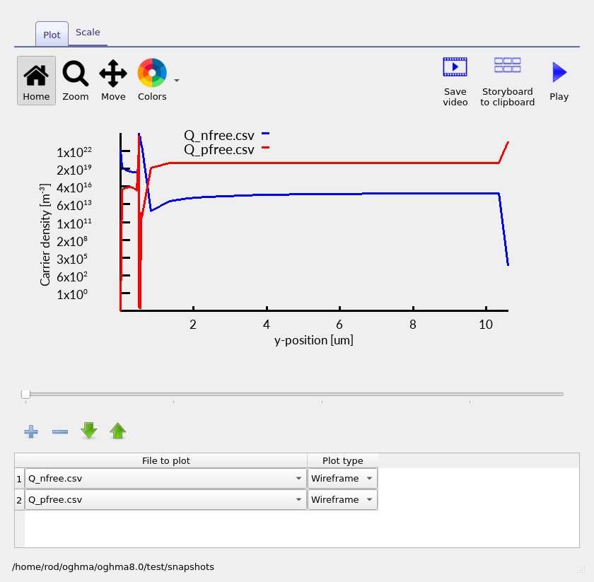
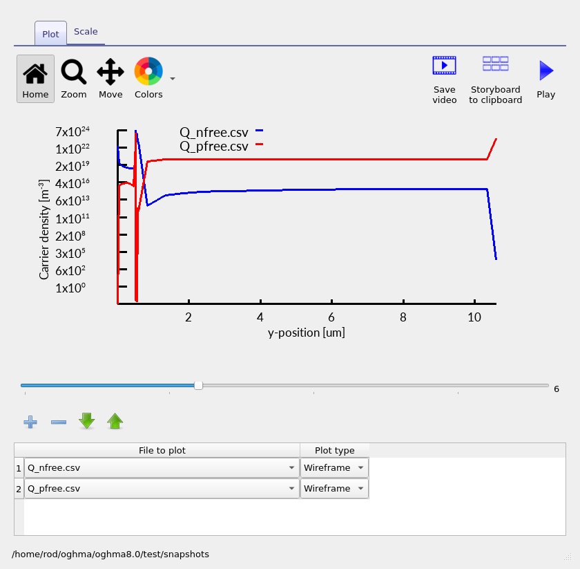
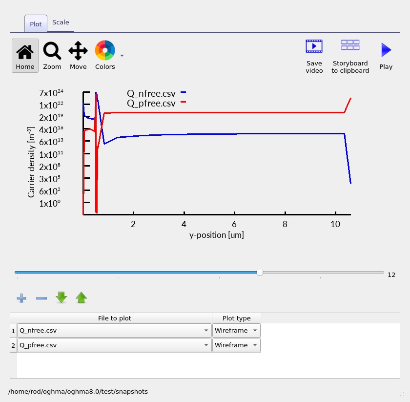
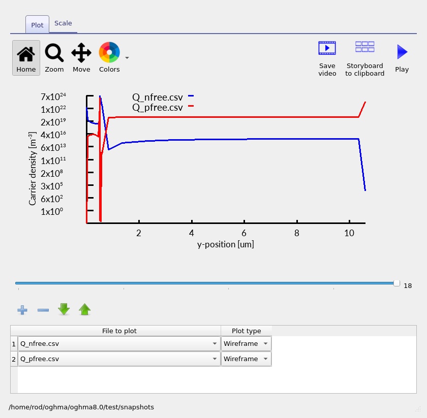
The carrier-density profiles show the local populations of electrons and holes. In the n+-Si region the equilibrium majority carriers are electrons; in the p-type silicon absorber they are holes. Under illumination, photogenerated minority carriers also contribute, and their concentrations depend on the local field, transport parameters, recombination and the operating point of the tandem.
The thin interconnection region is particularly interesting. Efficient recombination between the subcells depends on the availability of electrons and holes near the connection, and the local carrier densities can differ markedly from those in the thick absorber regions. Compare the carrier-density profiles with the band diagram to understand whether a change in concentration is associated with doping, a band offset, a local electric field or carrier injection.
9. Spatial optical generation: where the sunlight is absorbed
The top and bottom absorbers convert different parts of the sunlight into electron-hole pairs. OghmaNano calculates a wavelength-dependent optical field through the multilayer stack and converts absorption into a position-dependent photogeneration rate, G(y), supplied to the electrical continuity equations.
\[G(y)=\int \alpha(\lambda,y)\,\Phi(\lambda,y)\,d\lambda,\]where \(\Phi(\lambda,y)\) denotes an appropriately defined local spectral photon flux and \(\alpha(\lambda,y)\) is the wavelength-dependent absorption coefficient. In the complete transfer-matrix calculation, the electric-field distribution also accounts for optical interference and reflections at material boundaries.
Open the generation output and examine the saved profile (??). The illuminated perovskite is expected to absorb a substantial part of the higher-energy incident light, leaving a spectrally modified photon flux for the silicon bottom cell. The detailed profile depends on the assigned optical constants and layer thicknesses. The optical and electrical models therefore work together: generation creates carriers, while drift, diffusion and recombination determine how many are ultimately collected.
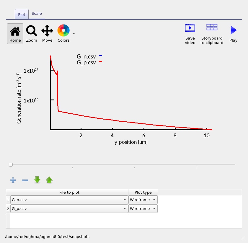
The generation profile is useful when changing perovskite thickness. A thicker top absorber can intercept more photons, but can also reduce the light available to the silicon. In a series-connected tandem the best thickness is not necessarily the one that maximises the current of either subcell in isolation; it is the one that provides a favourable balance of spectral absorption and electrical collection across the full device.
10. Suns-Voc and Suns-Jsc: exploring illumination intensity
After inspecting the one-sun J-V calculation, use the other simulation modes to ask how the tandem responds when the illumination changes. The Suns-Voc and Suns-Jsc modes are complementary: one examines the open-circuit voltage while the other examines the short-circuit current as the incident optical power is varied.
10.1. Suns-Voc
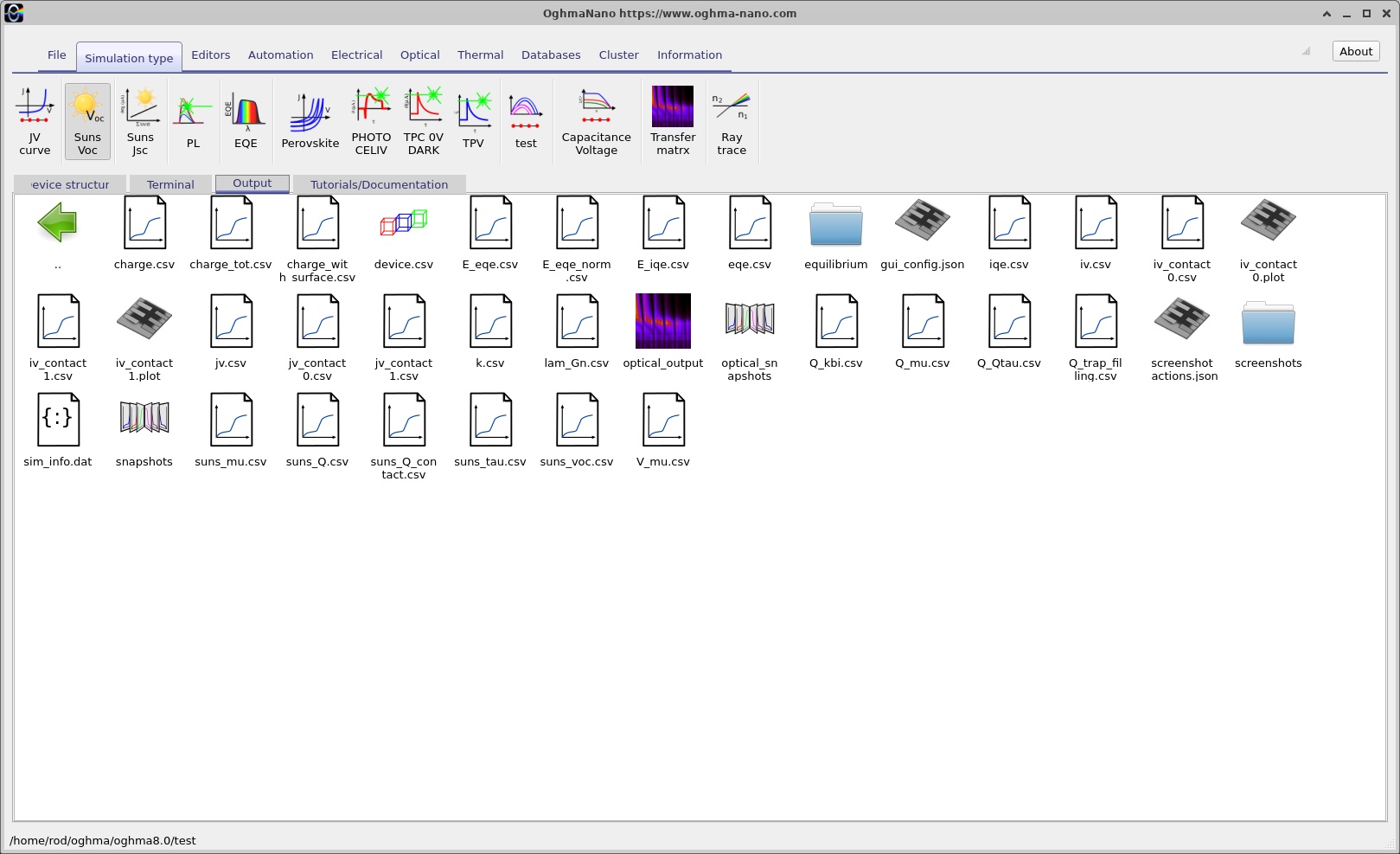
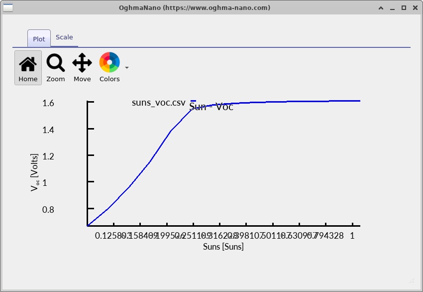
Choose Suns-Voc from the simulation selector and run the supplied intensity sweep. This calculation determines the terminal voltage for which the external current is zero at each illumination level. As photon generation increases, the nonequilibrium electron and hole populations generally grow, increasing quasi-Fermi-level separation and the measured open-circuit voltage.
For a simple diode approximation, the illumination dependence is approximately logarithmic:
\[V_{OC}\simeq \frac{n_{\mathrm{id}}k_BT}{q}\ln\!\left(\frac{J_{\mathrm{ph}}}{J_0}+1\right).\]Here \(n_{\mathrm{id}}\) is an effective ideality factor. For a tandem, the measured open-circuit voltage reflects both junctions and the interconnection. The resulting trend can be used to study how the coupled structure changes as carrier populations and recombination rates increase with illumination.
10.2. Suns-Jsc
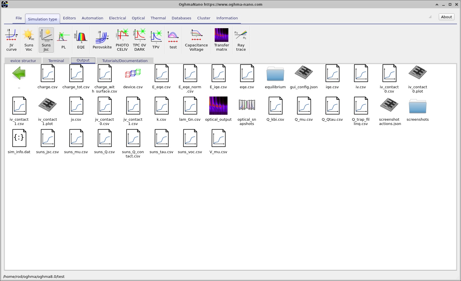
Choose Suns-Jsc and run its intensity sweep. At short circuit, the applied terminal voltage is approximately zero and the calculated external current is determined by how effectively the device absorbs photons and transports the resulting carriers to the terminals. Over an intensity range where collection efficiency does not change appreciably, the current density can increase approximately in proportion to the incoming photon flux:
\[|J_{SC}|\propto P_{\mathrm{sun}}.\]In a tandem, the short-circuit current can also be affected by how the two subcells share the common series current. If a change in illumination alters the internal carrier distributions or the operation of the recombination region, the trend may deviate from a simple proportional relationship. The Suns-Jsc result provides an additional way to investigate this behaviour without requiring a full J-V sweep at each light level.
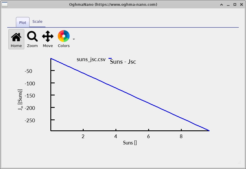
Compare the two intensity sweeps with the standard illuminated J-V curve. Suns-Voc isolates the voltage at zero terminal current; Suns-Jsc isolates current at zero external bias. Together they provide a broader view of how the tandem responds to changes in the available sunlight.
11. Exploring the optical field and absorption
The electrical results depend on the light absorbed in the perovskite and silicon. Open the Optical analysis window and inspect the available tabs (?? and ??). The example uses the transfer-matrix approach and an AM1.5G incident spectrum. Its optical wavelength mesh spans 300-1400 nm with 150 nominal wavelength points.
The transfer-matrix method treats each optically uniform layer as a medium with a complex refractive index, \(\tilde n=n+ik\). Forward- and backward-propagating waves interfere as they cross interfaces, so the optical intensity can vary with both wavelength and depth. This is important for tandem devices because the perovskite, transport layers, ITO electrodes and silicon all affect the spectrum reaching the bottom cell.
Use the optical tabs to move between the spatial field, wavelength and absorption-related views. The perovskite top cell is designed to take advantage of its larger bandgap, while the silicon cell is intended to absorb lower-energy light transmitted through the upper stack. Changes to the thickness of either absorber, or to the optical constants of an intervening layer, can alter the generated current in both subcells.
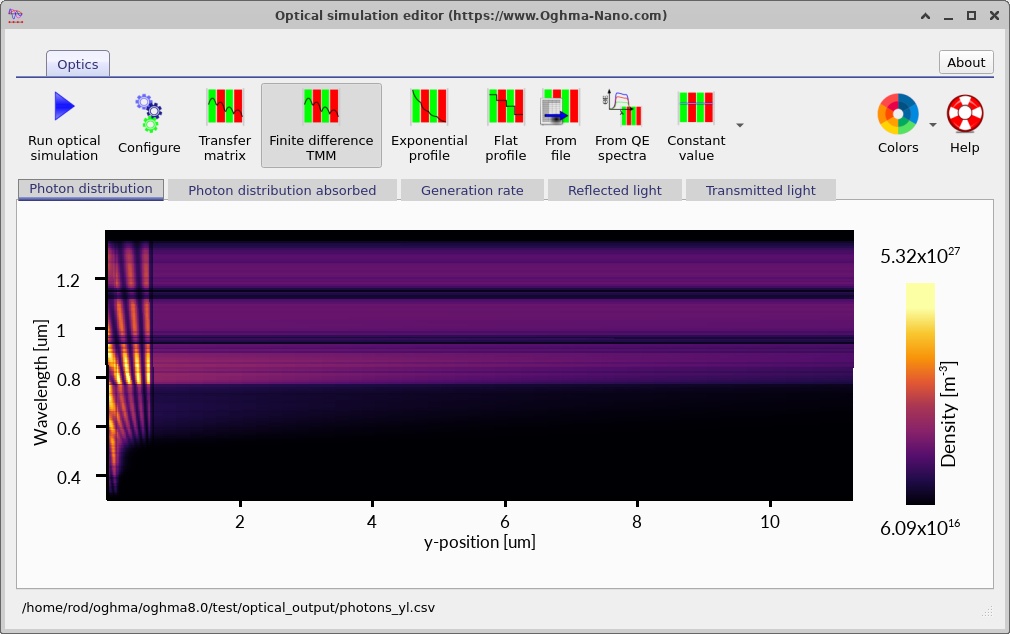
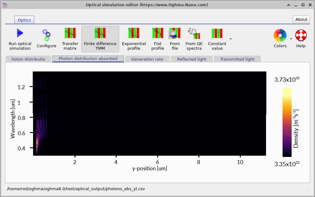
Notice that the optical calculation is distinct from the charge-transport calculation. Optical absorption determines where electron-hole pairs are created; their probability of reaching the contacts depends on the electrical model. Combining the two is what makes a drift-diffusion tandem simulation more informative than a purely optical absorption calculation.
12. Bringing the results together
The most useful way to interpret this example is to connect several views of the same device. The layer editor identifies the physical sequence of absorbers, transport layers and contacts. The doping and electrical parameter editors establish the semiconductor junctions and carrier transport properties. The optical calculation determines where sunlight generates charge. The band and carrier-density plots explain how the junctions and interconnection respond. Finally, the J-V and illumination-intensity curves show the combined electrical output.
For the two-terminal tandem, the important physical distinction is that the subcells are optically stacked and electrically series connected. The top absorber reshapes the spectrum seen by the bottom absorber, and the internal recombination junction enforces electrical continuity between their carrier currents. Changing a parameter in one subcell can therefore alter the behaviour of the complete device.
This example uses a deliberately compact silicon bottom cell and an effective interconnection model. Those choices make it practical as a tutorial for exploring the governing physics, inspecting numerical outputs and experimenting with tandem design. For quantitative comparison with a fabricated cell, the user would additionally select measured optical constants, appropriate interface models and calibrated electrical parameters for the actual structure.
13. Suggested investigations
Alternative approach: Combining independently simulated subcells
In this example, the perovskite and silicon subcells are connected through an explicit recombination layer. This allows their carrier transport to be calculated together within a single drift-diffusion simulation. An alternative is to solve the two photovoltaic junctions separately and construct the tandem current-voltage characteristic from their individual J-V curves. This approach is particularly useful when the strong recombination required at an idealised interconnection makes the coupled numerical problem difficult to converge.
The supplied tandem simulation is initially configured with all the semiconductor layers electrically active, allowing the complete device to be solved as a single drift-diffusion system. To simulate the two subcells independently, open the Layer Editor and modify the electrical configuration so that only one subcell is active at a time.
First, configure the perovskite top cell. Keep the perovskite
absorber and its associated charge-transport layers electrically active, and
change the silicon layers from Active to Other.
Next, use the Contacts Editor to position the electrical contacts
at the boundaries of the perovskite subcell. Run the illuminated J-V simulation
and save the resulting curve as jv_perovskite.csv.
Next, configure the silicon bottom cell. Change the perovskite
and its associated transport layers from Active to
Other, and restore the silicon layers to Active.
Move the electrical contacts to the boundaries of the silicon subcell, then
run the J-V simulation again. Save this curve as jv_silicon.csv.
Importantly, changing a layer from Active to Other removes it from the electrical drift-diffusion calculation but retains its optical properties. The optical generation calculation can therefore continue to account for absorption throughout the complete tandem stack, ensuring that the silicon subcell receives the light transmitted through the perovskite and upper transport layers. The two saved J-V curves can then be combined by interpolating their voltages at a common current density, as described below.
Two-terminal subcells connected in series carry the same current density (assuming equal active areas). Rather than finding an intersection between the two J-V curves, invert each curve to obtain its voltage as a function of current density. For every current density supported by both calculations, add the corresponding voltages:
\[ J_{\mathrm{pero}}=J_{\mathrm{Si}}=J, \qquad V_{\mathrm{stack}}(J)=V_{\mathrm{pero}}(J)+V_{\mathrm{Si}}(J). \]Interpolation gives the two subcell voltages on a common current-density grid. Only the current range covered by both simulations should be used; extrapolation outside that range can give misleading results. If the subcell J-V curves are not monotonic, their inverse may not be single-valued and the relevant operating branches must be treated separately.
It is often convenient to begin with a low series resistance and high shunt resistance, then add circuit losses to the combined result. With a positive current-density convention for power delivered by the cell, a total area-normalised series resistance, \(R_s\), gives
\[ V_{\mathrm{terminal}}(J)=V_{\mathrm{stack}}(J)-JR_s. \]A shunt placed across the complete tandem is a parallel current pathway, not an additional voltage drop. With area-normalised shunt resistance \(R_{\mathrm{sh}}\), the terminal current density is
\[ J_{\mathrm{terminal}}=J-\frac{V_{\mathrm{terminal}}}{R_{\mathrm{sh}}}. \]Shunts associated with an individual subcell should instead be included in that subcell's electrical model. The same applies to any series losses already included in its calculated J-V curve: avoid counting the same resistance twice. Resistances in the equations above are area-normalised (\(\Omega\,\mathrm{m^2}\)) when current is expressed as a density in \(\mathrm{A/m^2}\).
The Python example below (also available as a separate script) reads two CSV files containing voltage (V) and current density (A/m²), interpolates both voltages at matching currents, and writes the combined tandem characteristic. It also accepts optional series and whole-tandem shunt resistances. The script assumes positive current density corresponds to power delivered by the cell; invert the sign of exported data first if the OghmaNano plot uses the opposite convention.
Python example: combining the two J-V curves
#!/usr/bin/env python3
"""Combine two photovoltaic subcell J-V curves at equal current density.

Input CSV files: two columns, voltage_V,current_density_A_m2.
Positive J means current delivered by a photovoltaic subcell.
Resistances are area-normalised in ohm*m^2.
"""
import argparse
import numpy as np


def load_jv(filename):
    data = np.loadtxt(filename, delimiter=",", skiprows=1, ndmin=2)
    if data.shape[1] != 2 or data.shape[0] < 2:
        raise ValueError(f"{filename}: expected at least two rows with V,J")
    voltage, current = data[:, 0], data[:, 1]
    if not (np.isfinite(voltage).all() and np.isfinite(current).all()):
        raise ValueError(f"{filename}: non-finite values")
    order = np.argsort(voltage)
    voltage, current = voltage[order], current[order]
    if not np.all(np.diff(voltage) > 0):
        raise ValueError(f"{filename}: repeated voltage values")
    dcurrent = np.diff(current)
    if not (np.all(dcurrent > 0) or np.all(dcurrent < 0)):
        raise ValueError(f"{filename}: J(V) must be strictly monotonic to invert")
    order = np.argsort(current)
    return current[order], voltage[order]


def combine(top_file, bottom_file, output_file, rs, rsh, points):
    jt, vt = load_jv(top_file)
    jb, vb = load_jv(bottom_file)
    jmin = max(jt[0], jb[0])
    jmax = min(jt[-1], jb[-1])
    if jmax <= jmin:
        raise ValueError("The subcell J-V curves have no shared current interval")
    j = np.linspace(jmin, jmax, points)
    vtop = np.interp(j, jt, vt)
    vbottom = np.interp(j, jb, vb)
    vstack = vtop + vbottom
    vterminal = vstack - j * rs
    # Optional shunt connected across the *complete tandem terminal pair*.
    jterminal = j - vterminal / rsh if np.isfinite(rsh) else j.copy()
    result = np.column_stack((vterminal, jterminal, j, vtop, vbottom))
    np.savetxt(output_file, result, delimiter=",", comments="",
               header="voltage_V,current_density_A_m2,stack_current_density_A_m2,top_voltage_V,bottom_voltage_V")
    print(f"Saved {points} points to {output_file} (shared J: {jmin:g} to {jmax:g} A/m^2)")


if __name__ == "__main__":
    parser = argparse.ArgumentParser(description=__doc__)
    parser.add_argument("top", help="Top-cell CSV (voltage_V,current_density_A_m2)")
    parser.add_argument("bottom", help="Bottom-cell CSV (voltage_V,current_density_A_m2)")
    parser.add_argument("-o", "--output", default="tandem_jv.csv")
    parser.add_argument("--rs", type=float, default=0.0,
                        help="Area-specific series resistance in ohm*m^2")
    parser.add_argument("--rsh", type=float, default=float("inf"),
                        help="Area-specific external tandem shunt in ohm*m^2")
    parser.add_argument("--points", type=int, default=300)
    args = parser.parse_args()
    if args.rs < 0 or args.rsh <= 0 or args.points < 2:
        parser.error("Require rs >= 0, rsh > 0, points >= 2")
    combine(args.top, args.bottom, args.output, args.rs, args.rsh, args.points)
Save the script as combine_tandem_jv.py and run it with:
python3 combine_tandem_jv.py perovskite.csv silicon.csv -o tandem_jv.csv \
    --rs 1e-4 --rsh 10
This series-coupled approach retains the separately calculated carrier transport, recombination and optical generation in each absorber, while approximating the interconnection as an ideal electrical series connection plus any specified circuit losses. It does not explicitly resolve tunnelling, charge accumulation or other microscopic effects within a real recombination junction.