Optical detectors
1. Introduction
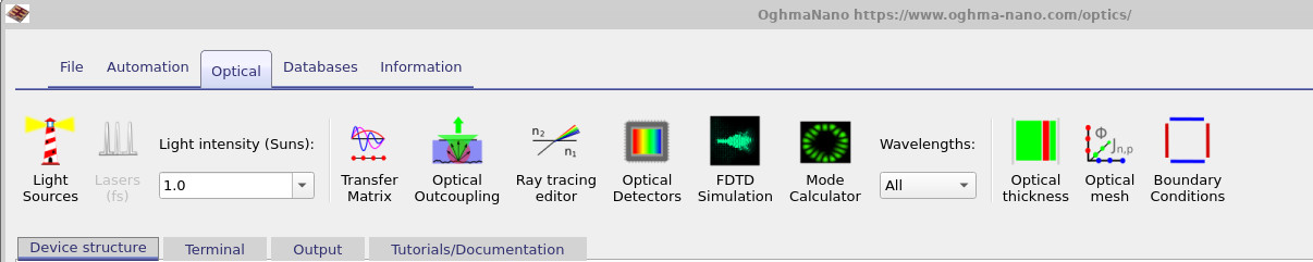
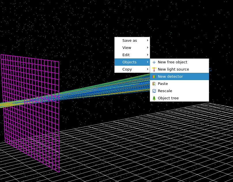
In OghmaNano, optical detectors are used to measure light as it propagates through an optical system. Detectors are defined using the Optical Detectors Editor, which can be opened from the Optical ribbon in the main window (see Figure ??).
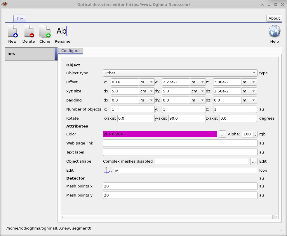
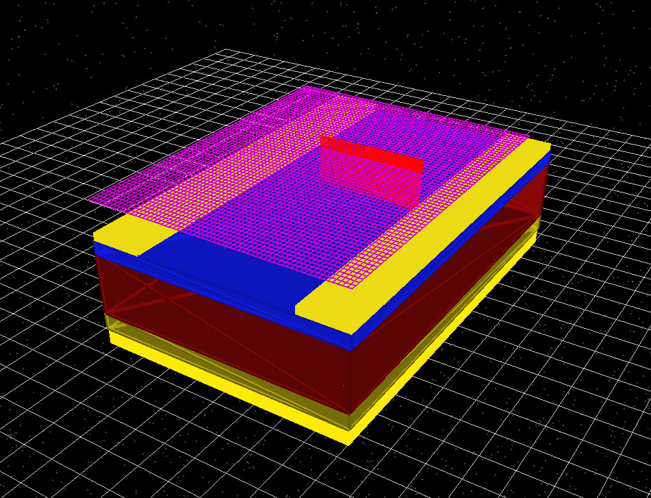
The Optical Detectors Editor is shown in ??. An optical detector in OghmaNano is a two-dimensional surface placed anywhere in the simulation domain. Conceptually, it behaves like an idealised CCD camera: it counts photons passing through it and records their spectral and spatial distribution.
Detectors do not absorb, reflect, or scatter light. They are mathematically transparent and do not perturb the optical field. Rays, waves, or photons pass through the detector unmodified; the detector simply records what crosses its surface.
2. Detector geometry and resolution
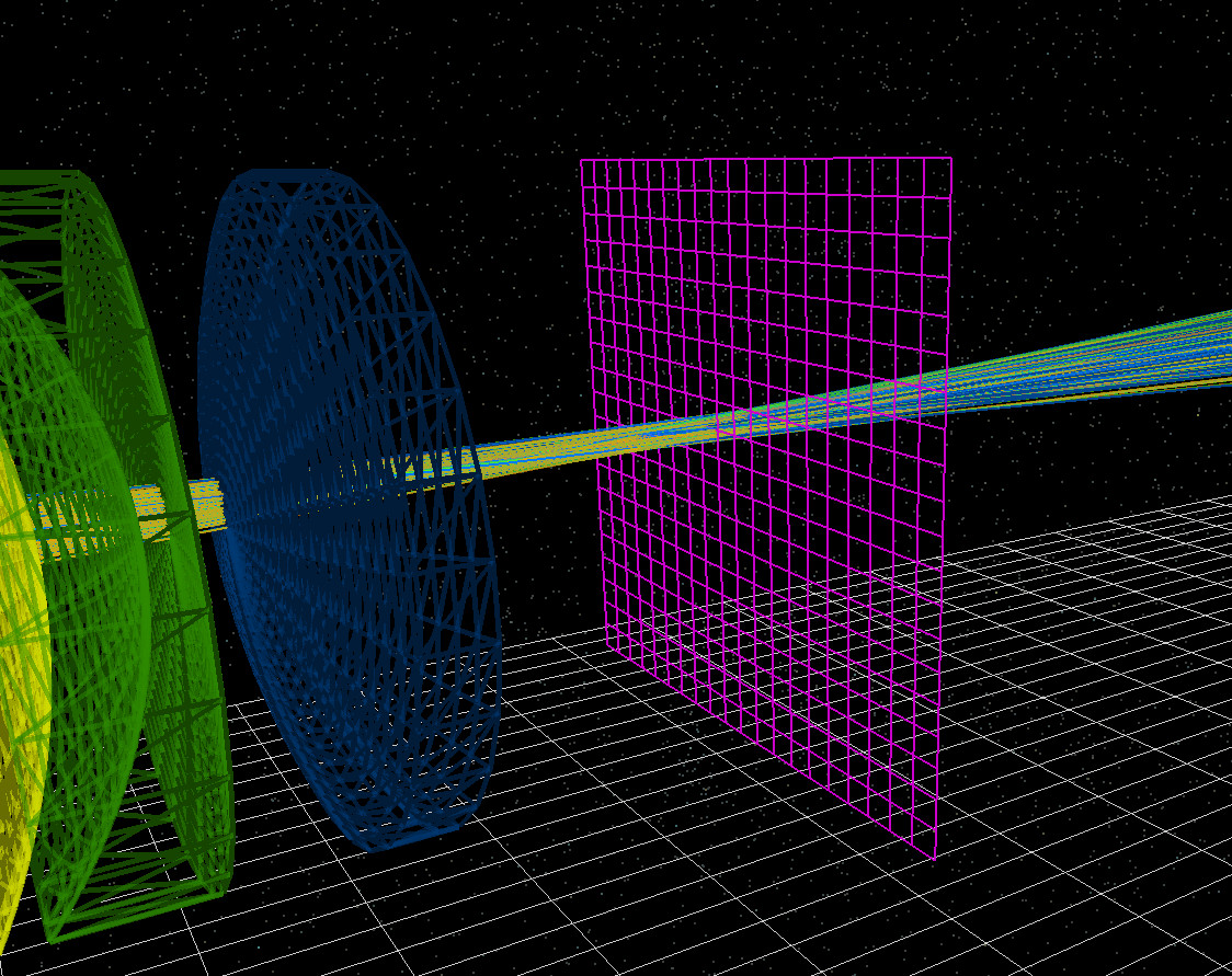
A detector is defined by its position, orientation, and lateral size (\(dx\) and \(dy\)). The thickness \(dz\) is irrelevant, as the detector is treated as a purely two-dimensional surface. The detector can be rotated about the \(x\), \(y\), and \(z\) axes, allowing it to face in any direction. This makes it possible to capture transmitted, reflected, or escaping light in arbitrary geometries. Detectors can also be repositioned interactively by dragging them within the 3D scene.
Under the Detector section of the configuration panel, the parameters Mesh points x and Mesh points y define the number of spatial bins used across the detector surface. These correspond directly to the number of pixels in a CCD sensor, controlling the spatial resolution of the recorded data. Multiple detectors may be placed in a single simulation. Each detector operates independently and produces its own set of output files.
3. Detector examples
4. Outputs
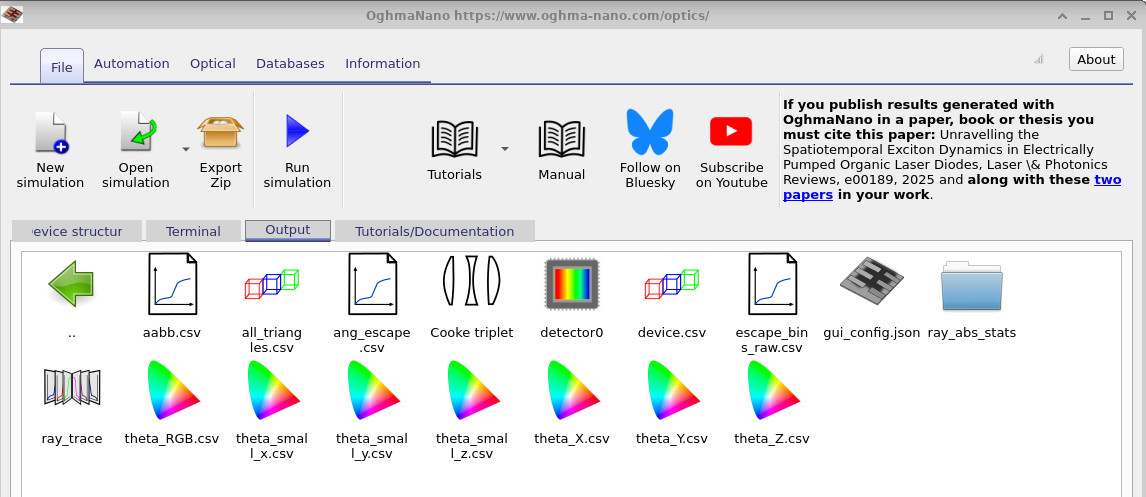
When you open a detector’s output folder you will typically see four files
(see Figure ??):
detector_abs0.csv, detector_efficiency0.csv,
detector_input0.csv, and RAY_image.csv.
Together these describe (i) the spatial distribution of detected light and
(ii) the spectral throughput from the source to the detector.
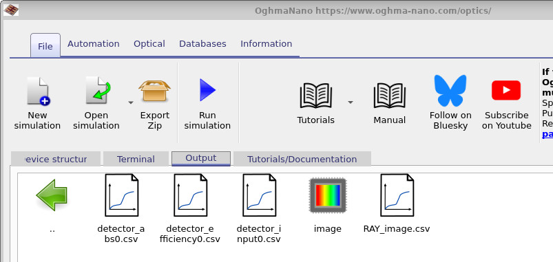
RAY_image.csv is a spatially resolved image of what the detector receives
(conceptually a CCD frame). In ray-tracing mode it is usually generated by tracing
three representative wavelengths (nominally “R”, “G”, and “B”) and mapping them directly
to an RGB image. In non-ray-tracing workflows, or when you trace a broader wavelength set,
OghmaNano converts the detected spectrum into displayable RGB using standard human visual
colour-response functions (so the colour is an appearance estimate of what an eye would see,
rather than a literal three-wavelength render). In practice, for EL/PL spectra you should
trace many wavelengths; three-colour RGB is fine for quick optics visualisation, but it is too
sparse for emission spectra.
The remaining three files form a simple “input → detected → efficiency” chain:
-
detector_abs0.csv(??): the available source spectrum that could, in principle, have reached the detector. This is the distribution of emitted rays/photons versus wavelength before geometry and absorption decide what actually arrives. -
detector_input0.csv(??): the spectrum of rays/photons that actually reach and pass through the detector surface (reported as counts). Material absorption and clipping modify this. In the example shown, glass removes the UV part of the spectrum, producing a sharp reduction at short wavelengths. -
detector_efficiency0.csv(??): the detection probability (percentage) versus wavelength, computed as \[ \eta(\lambda)=100\times\frac{I_{\text{det}}(\lambda)}{I_{\text{avail}}(\lambda)} =100\times\frac{\texttt{detector_input0.csv}}{\texttt{detector_abs0.csv}}. \] Interpreted physically: if a ray/photon is emitted at wavelength \(\lambda\), what fraction of those emissions end up crossing the detector?
RAY_image.csv).
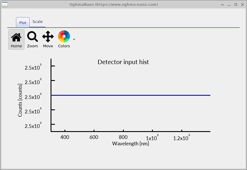
detector_abs0.csv).
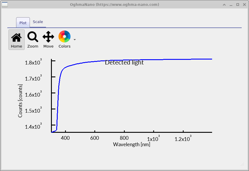
detector_input0.csv).
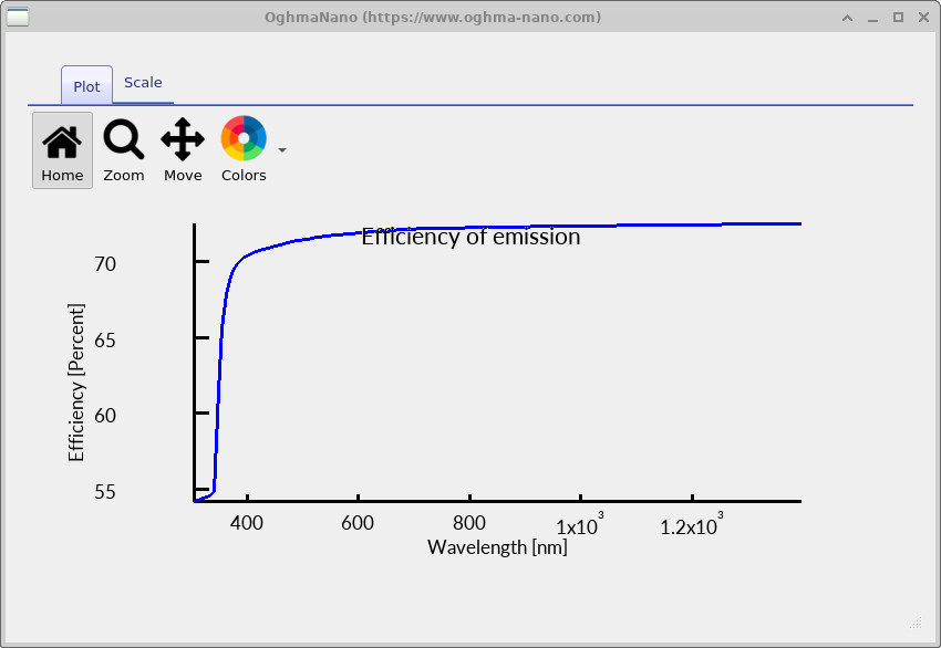
detector_efficiency0.csv).