Optical Light Sources and Illumination Spectra

1. Introduction

In OghmaNano, light sources are used to define the illumination spectra that enter an optical simulation. Any incident optical power, whether it originates from sunlight, a laser, a lamp, or a user-defined spectrum, is introduced into the simulation through a light source. For example, a standard AM1.5G solar spectrum, a monochromatic laser, or a measured experimental spectrum can all be represented using the Light Source Editor.

The light source system is shared across all optical solvers in OghmaNano, providing a consistent way to define illumination conditions regardless of the simulation method being used. The same light source definitions can therefore be applied to transfer matrix simulations, finite-difference time-domain (FDTD) simulations, and ray tracing simulations. This ensures that different optical models can be compared directly under identical illumination conditions.

This page explains how to create, combine, and configure light sources, apply optical filters, and control the direction and spatial origin of illumination within OghmaNano.

2. Opening the light source editor

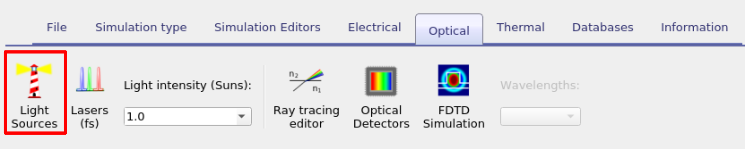
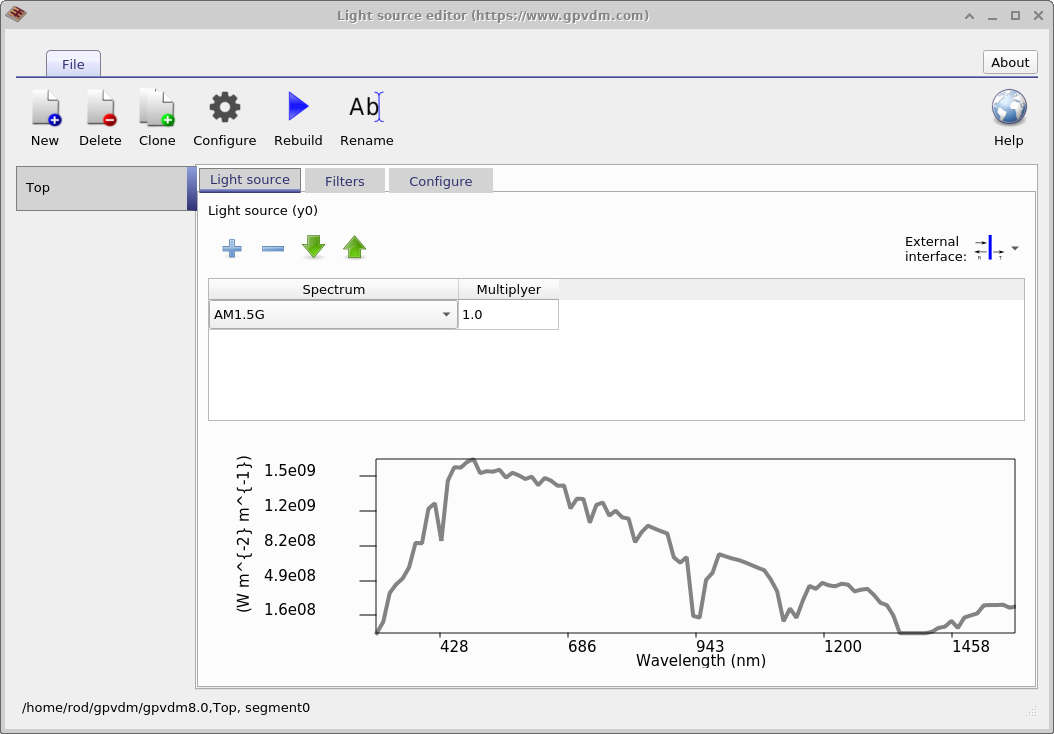
The Light Source Editor is accessed from the Optical ribbon in the main window (see Figure ??). Once open it looks like ??. A light source in OghmaNano is defined by its illumination spectrum. For example, you can configure a source to emit the standard AM1.5G spectrum. Multiple spectra can then be combined in the Light Source tab. This makes it possible to superimpose different spectra, such as AM1.5G illumination together with the emission of a fluorescent tube. The relative intensity of each source is set using the multiplier column, which scales the contribution of each spectrum.

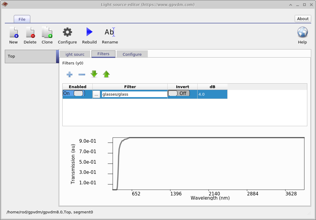
Optical filters, managed in the Filters tab (??), are applied to the combined spectrum rather than to individual light sources. Filters represent materials that absorb or block certain wavelength ranges — for example, simulating a thick glass layer that blocks sunlight below 300 nm. They can be enabled or disabled with the Enable switch, their material selected, and the attenuation strength specified in dB.

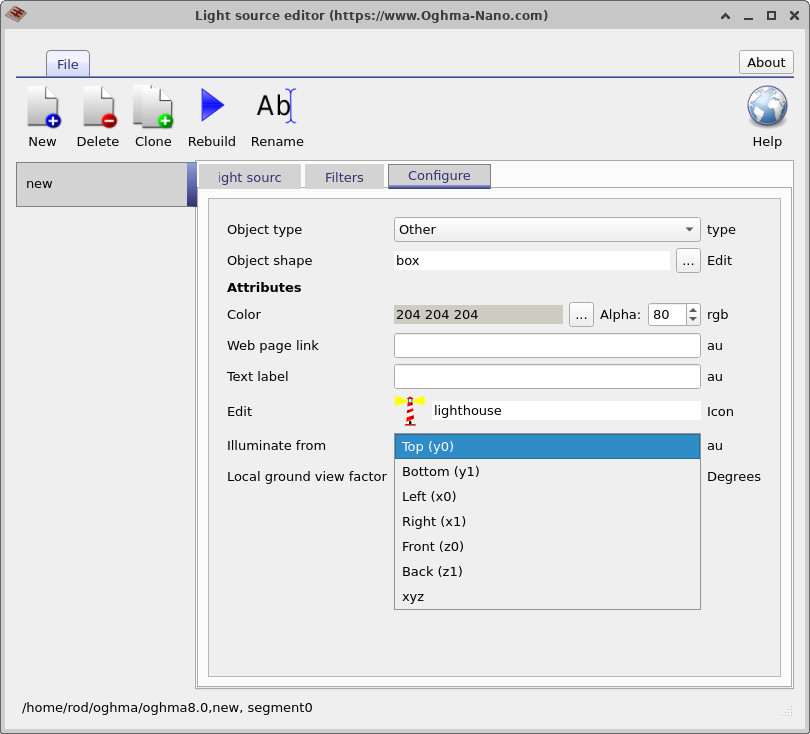
3. Light Source Orientation

In OghmaNano, each light source can be configured to illuminate the simulation from a specific direction or from an arbitrary position in three-dimensional space. The available source directions are top (y0), bottom (y1), left (x0), right (x1), front (z0), back (z1), and an arbitrary xyz position. Example source configurations are shown in Figures ??, ??, ??, and ??.

The selected light source orientation is automatically passed to the optical solver being used. OghmaNano employs a common light source framework across the transfer matrix method, FDTD, and ray tracing solvers, allowing the same illumination conditions to be reused across different optical simulation techniques.

• Top (y0): Light enters through the top boundary of the simulation domain. This is the most common configuration for solar-cell simulations and is frequently used with the transfer matrix method. An example is shown in ??.
• Bottom (y1): Light enters through the bottom boundary of the simulation domain. This configuration is commonly used when modelling illumination through a substrate or when simulating bifacial devices. An example is shown in ??.
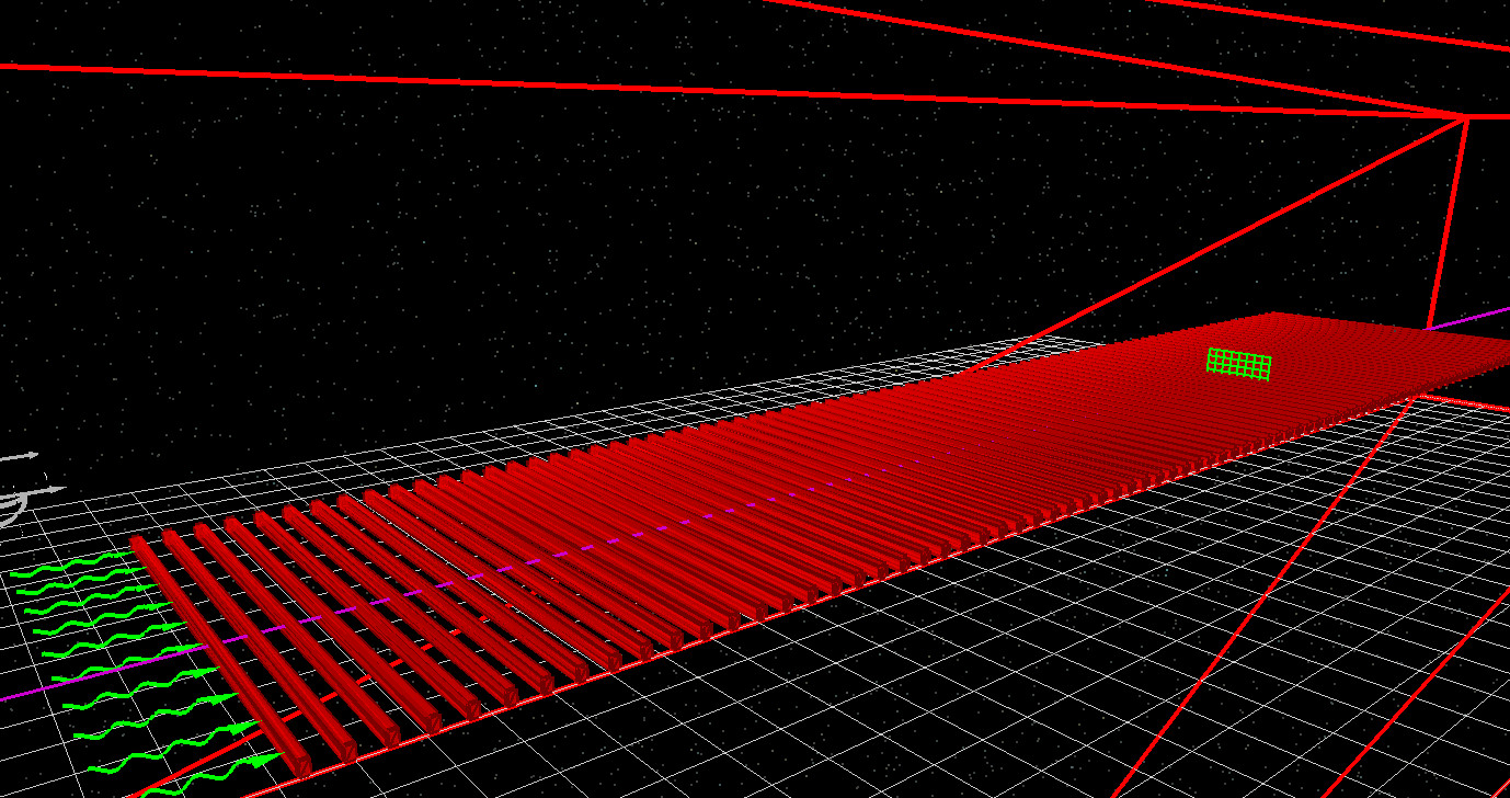
• Left (x0) and Right (x1): Light enters through the left- or right-hand boundaries of the simulation domain. These source types are useful when modelling waveguide structures, diffraction gratings, edge-coupled devices, and lateral illumination geometries. An example of side illumination is shown in ??.
• Front (z0) and Back (z1): Light enters through the front or rear z-boundaries of the simulation domain. These options are primarily used in three-dimensional optical simulations where illumination is required along the z-axis.
• xyz Position: The light source is placed at an arbitrary location within the three-dimensional simulation space. This mode is generally preferred for FDTD and ray tracing simulations because it allows complete control over source position and illumination geometry. An example is shown in ??.

The available source types depend on the optical solver being used. For transfer matrix simulations, illumination is applied through one of the simulation boundaries (x0, x1, y0, y1, z0, or z1). Arbitrary xyz sources are not supported because the transfer matrix method requires well-defined boundary conditions and a known propagation direction. In contrast, both FDTD and ray tracing simulations support arbitrary xyz light sources and these are generally the preferred source type for complex three-dimensional optical systems.

Multiple light sources may be combined within a single simulation. For example, a device may be illuminated simultaneously from the top (y0) and bottom (y1) surfaces to model bifacial solar-cell operation. Similarly, sources entering from different directions can be combined to represent diffuse illumination, multiple lamps, reflected light, or complex experimental geometries.

4. Configuring xyz Light Sources

When illumination is applied through one of the simulation boundaries (x0, x1, y0, y1, z0, or z1), OghmaNano assumes a uniform plane-wave source propagating normal to the selected boundary. For many optical simulations this is sufficient. More complex optical systems, however, often require a source to be positioned at a specific location within the simulation domain. This is achieved using an xyz light source.

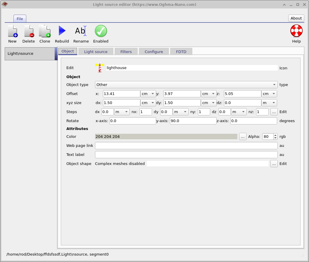
An xyz light source is treated as a standard OghmaNano object and therefore shares the same positioning and geometry controls used throughout the optical simulation environment. These parameters are available from the Object tab of the Light Source Editor, shown in ??. The same dialog can also be opened directly from the 3D simulation window by right-clicking on the light source and selecting Edit Object.

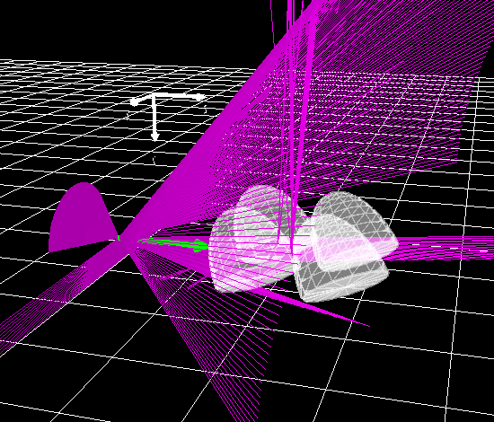
The object parameters define the position, size, and orientation of the emitting surface. The Offset values specify the x, y, and z coordinates of the source, while the xyz size parameters define its physical dimensions. In practice, an xyz light source is represented as an emitting plane with finite dimensions in x and y and negligible thickness in z. This makes it possible to model square or rectangular illumination sources located anywhere within the simulation domain. Rotation parameters can be used to orient the emitting plane relative to the surrounding optical system.

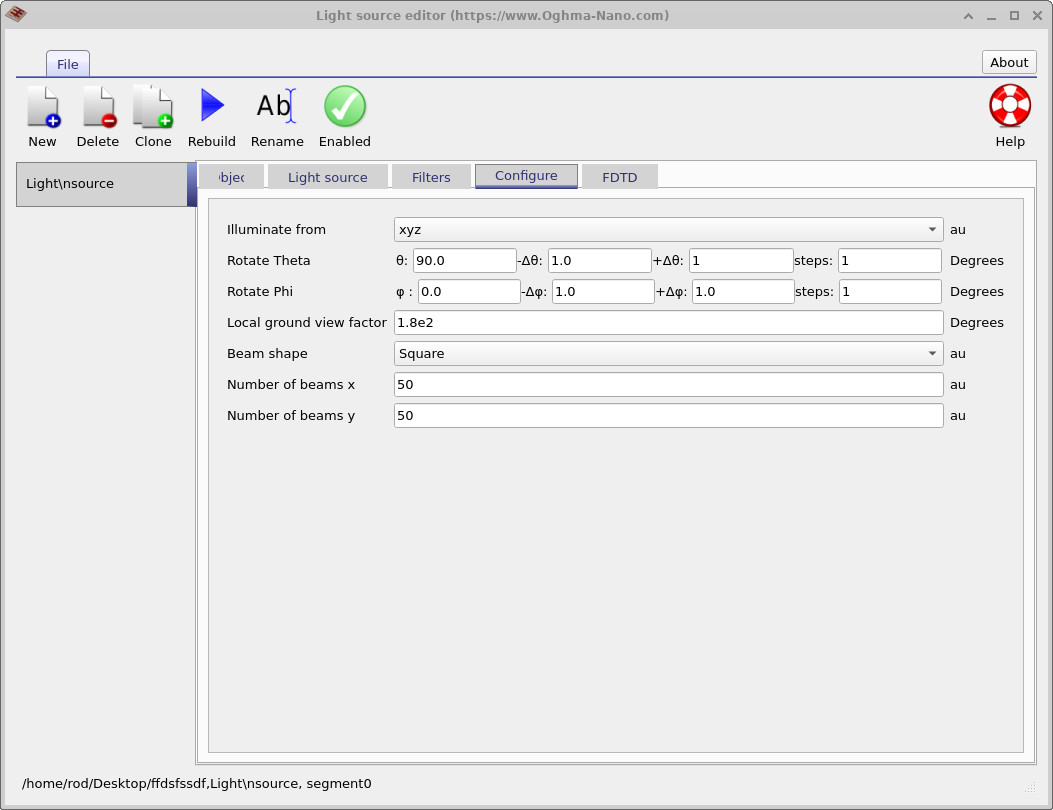
The optical emission characteristics of the source are configured separately using the Configure tab shown in ??. Here, the angles θ and φ define the direction of propagation, while the associated sweep parameters (Δθ, Δφ, and the number of steps) allow light to be emitted over a range of angles. In ray-tracing simulations this can be used to generate cones, fans, or other angular distributions of rays from a single source.

The Beam shape parameter controls the spatial distribution of rays across the emitting plane. The Number of beams x and Number of beams y settings determine how densely the source is sampled. In the example shown in ??, a 50 × 50 beam grid launches 2500 rays from the source plane. Increasing the beam density generally improves sampling accuracy, although at the cost of additional computation time.

The combination of arbitrary positioning, source geometry, and angular control makes xyz light sources particularly useful in ray-tracing and FDTD simulations. Typical applications include modelling lasers, LEDs, optical fibres, waveguides, imaging systems, and other optical assemblies where both the location and emission pattern of the source are important parts of the overall design.

5. FDTD Light Sources

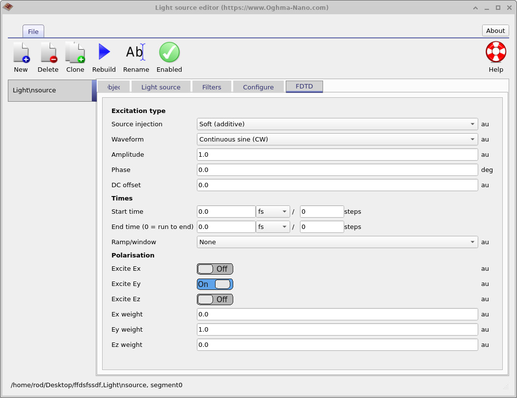
Unlike the optical light source settings described in the previous sections, FDTD simulations require additional source parameters that control how electromagnetic fields are injected into the simulation domain. These settings are available from the dedicated FDTD tab shown in ??.

FDTD light sources have a number of properties that are not normally required by transfer matrix or ray-tracing simulations. For example, it is necessary to specify the source injection method, waveform type, amplitude, phase, timing, and field polarisation. These parameters determine how the source interacts with the FDTD mesh and how electromagnetic energy is introduced into the simulation.

Because these settings are specific to the finite-difference time-domain method, they are ignored when running transfer matrix, ray-tracing, or other optical simulations. The tab is only used when an FDTD simulation is being performed.

A detailed description of each FDTD source parameter is provided in the dedicated FDTD light source documentation. For a complete discussion of source injection methods, waveforms, timing controls, and polarisation settings, see FDTD Light Sources.

6. Local Ground View Factor

The local ground view factor describes how much of the surrounding ground surface is visible to a given point on the device. It is relevant when considering optical simulations that include reflected or scattered light from the ground plane. In other words, it accounts for the fraction of the diffuse radiation field that originates from the ground beneath the device.

The factor is defined as

\[ F_{\text{ground}} = \sin^2\!\left(\frac{\theta_t}{2}\right) = \frac{1 - \cos(\theta_t)}{2}, \]

where \(\theta_t\) is the tilt angle of the device with respect to the horizontal plane. A horizontal device (\(\theta_t = 0\)) sees no ground, giving \(F_{\text{ground}} = 0\). A vertical device (\(\theta_t = 90^\circ\)) has a ground view factor of 0.5, since half of its diffuse environment is the ground and half is the sky.

This parameter can be set in the Configure tab. It is typically used in cases where ground-reflected light (albedo) makes a non-negligible contribution to the illumination — for example, in outdoor solar cell simulations, building-integrated photovoltaics, or devices exposed to highly reflective surfaces such as snow or white roofing.

7. Conclusion

OghmaNano provides a unified light source framework across transfer matrix, ray-tracing, and FDTD simulations. Light sources can be used to define arbitrary illumination spectra, combine multiple optical sources, apply optical filters, and control the position, orientation, and angular distribution of incident light. This common framework allows the same illumination conditions to be reused across different optical solvers, simplifying the construction and comparison of optical simulations.

For solver-specific details, see the documentation for transfer matrix, ray-tracing, and FDTD simulations.