Understanding Output Files in OghmaNano

When you run a simulation in OghmaNano, the software generates a large collection of output files describing the electrical, optical, thermal, and structural state of the simulated device. These files include JV curves, carrier densities, recombination rates, electric fields, optical spectra, transient data, and snapshots of the internal device state.

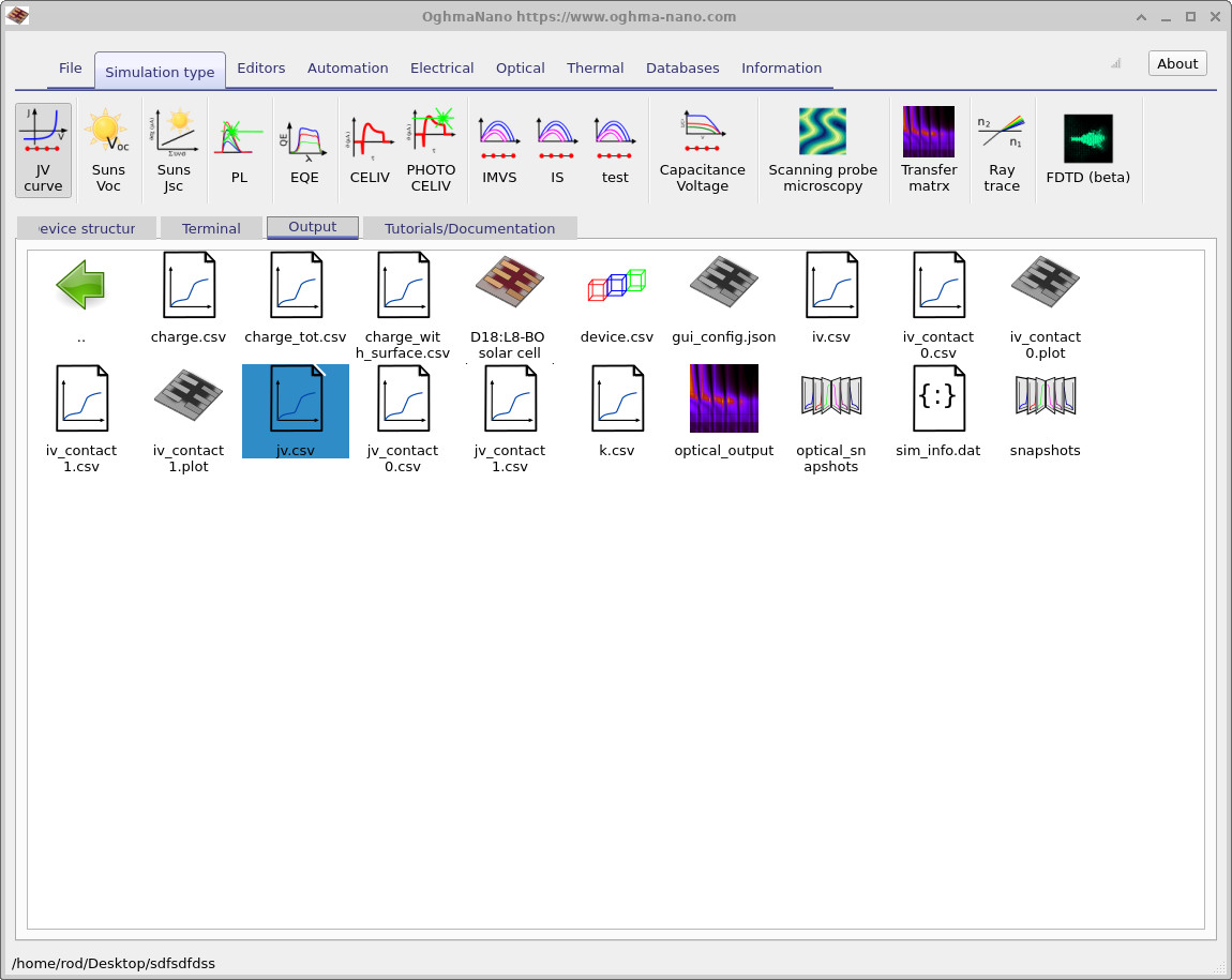
Rather than presenting these files as generic filesystem objects, OghmaNano provides a curated graphical interface designed to make browsing simulation data easier. The software attempts to understand the contents of each file and automatically displays it using the appropriate viewer. For example, JV curves appear as graph icons, device structures are shown as 3D models, and optical snapshots are displayed as image stacks.

The simulation output directory is shown in ??. When the file jv.csv is double-clicked, OghmaNano automatically displays the current density–voltage curve associated with the dataset.

Simulation output directory showing generated files including jv.csv. — The simulation output directory containing generated output files including `jv.csv`.

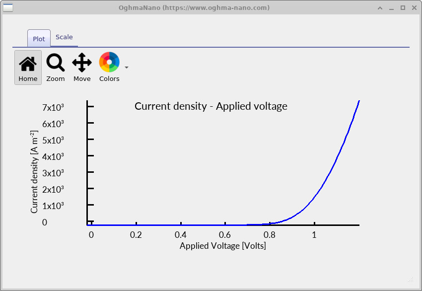
JV curve automatically displayed from jv.csv. — The JV curve automatically displayed when `jv.csv` is opened.

Internally, these files are stored either as standard human-readable CSV files or in a compact binary format. This means the data can be processed directly using external tools such as Python, MATLAB, GNU Octave, Excel, or custom analysis software.

CSV and binary output formats

OghmaNano supports two different methods for storing simulation output data:

Human-readable CSV files
Compact binary files

The CSV format is easy to inspect manually and can be opened directly in standard software packages. Binary files are substantially more compact and faster to read and write, making them preferable for large simulations.

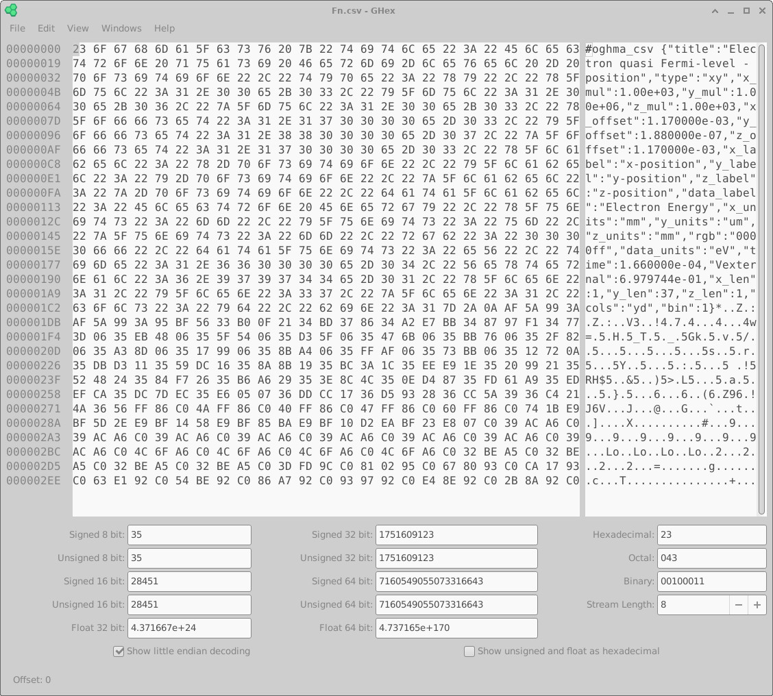
Examples of both formats are shown in ?? and ??.

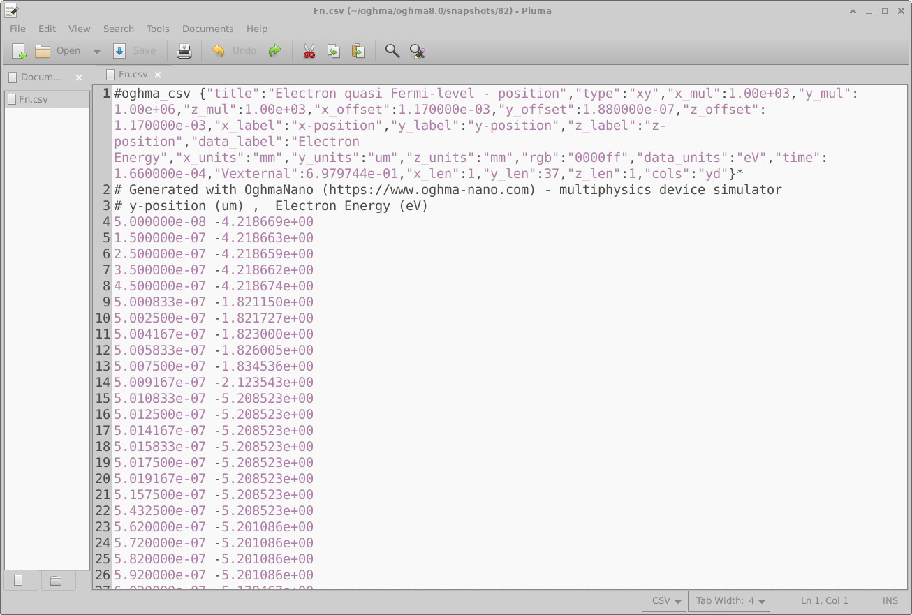
Example OghmaNano CSV output file. — Example CSV output file generated by OghmaNano containing metadata and human-readable numerical data.

Binary OghmaNano output file. — The same dataset stored in compact binary format.

At the start of every OghmaNano dataset is a metadata section beginning with:

#oghma_csv

This identifies the file as an OghmaNano-compatible dataset. Immediately after this marker is a JSON metadata header describing the contents of the file.

The JSON header tells OghmaNano how the data should be interpreted and plotted. Because the header uses standard JSON syntax, it can also be parsed directly using external software libraries.

Typical fields found in an OghmaNano JSON output header.
Field	Description
`title`	Title of the dataset or graph.
`type`	Dataset type (for example xy, xyz, image, or vector field).
`x_mul`, `y_mul`, `z_mul`	Scaling multipliers applied to the axes.
`x_label`, `y_label`, `z_label`	Axis labels used when plotting the dataset.
`x_units`, `y_units`, `z_units`	Physical units associated with each axis.
`data_label`	Description of the stored data values.
`data_units`	Units associated with the stored data.
`time`	Simulation time or applied bias point.
`rgb`	Preferred plotting colour.
`cols`	Column ordering inside the file.

In CSV mode, the numerical values are stored as standard human-readable text. This makes the files easy to inspect manually but increases both file size and disk I/O overhead.

In binary mode, the numerical values are stored directly as binary floating-point numbers. This significantly reduces file size and improves performance, especially for large 2D and 3D simulations, transient calculations, optical snapshots, and FDTD simulations.

Switching between human-readable and binary format

The output format used by OghmaNano can be configured from the Automation ribbon shown in ??.

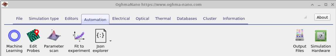
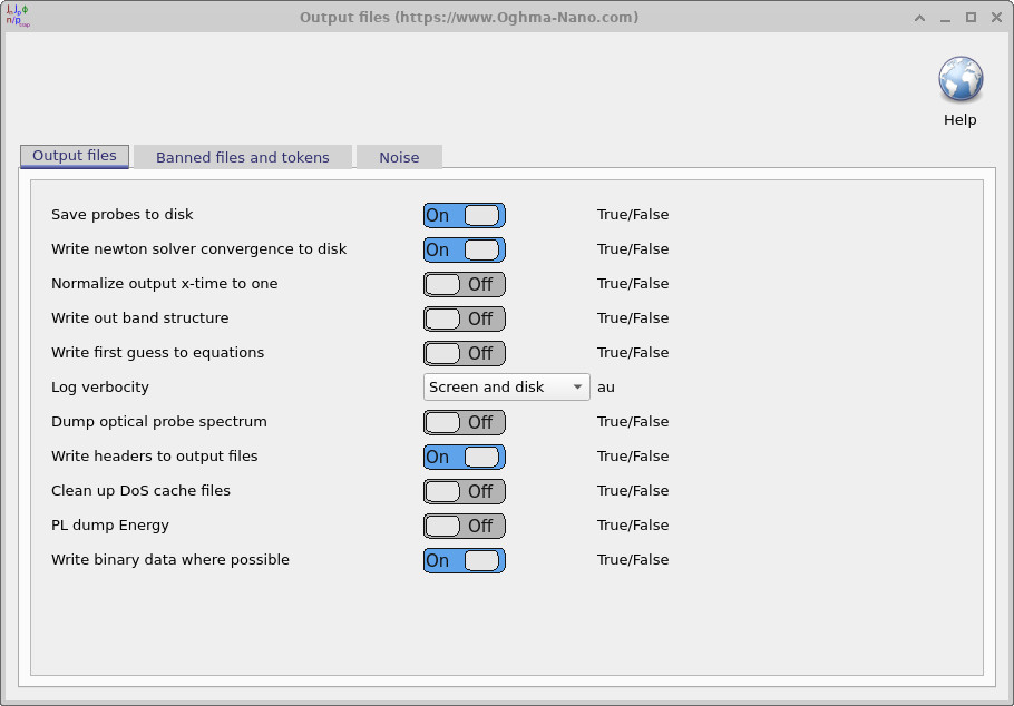
Automation ribbon in OghmaNano. — The Automation ribbon containing the *Output Files* configuration button.

Output file configuration window. — The output configuration window controlling how datasets are written to disk.

The option:

Write binary data where possible

controls whether OghmaNano attempts to store datasets using compact binary encoding.

Enabled: OghmaNano writes binary datasets where possible.
Disabled: OghmaNano writes standard human-readable CSV files.

If you are only viewing datasets inside OghmaNano itself, there is usually no visible difference because the software transparently handles both formats internally.

However, if you intend to process the data using external software, it is important to choose the appropriate storage format.

Processing files externally

One of the strengths of OghmaNano’s output system is that the generated datasets can be processed directly using external software.

Typical workflows include:

Loading JV curves into Excel for plotting.
Processing charge densities using Python and NumPy.
Importing spectra into MATLAB or GNU Octave.
Performing automated parameter extraction.
Generating publication-quality figures externally.

Because the metadata header contains units, scaling factors, labels, and plotting information, external scripts can automatically determine how datasets should be interpreted.

💡 Tip: For large simulations or parameter sweeps, enabling binary output can substantially reduce disk usage and improve simulation performance by reducing disk I/O overhead.