Understanding Snapshots in OghmaNano

What are snapshots?

When you run a simulation in OghmaNano, the software can optionally store intermediate simulation outputs called snapshots. Snapshots are effectively the state of the simulation stored at different points during the calculation.

For example:

• For a JV simulation, snapshots may be written at each voltage step along the JV curve.
• For a transient simulation, snapshots may be written at each timestep.
• For FDTD simulations, snapshots may store the optical field distribution as the electromagnetic wave propagates through the simulation domain.

Snapshots provide a way to peer inside the simulation while it is evolving. Rather than only examining the final output, snapshots allow you to inspect how the internal device state changes throughout the calculation.

Snapshot generation can usually be turned on or off directly inside the editor window associated with the simulation type being used. For example, the JV editor window shown in ?? contains options controlling snapshot generation.

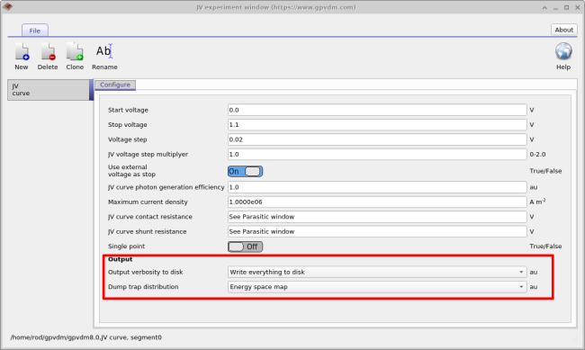
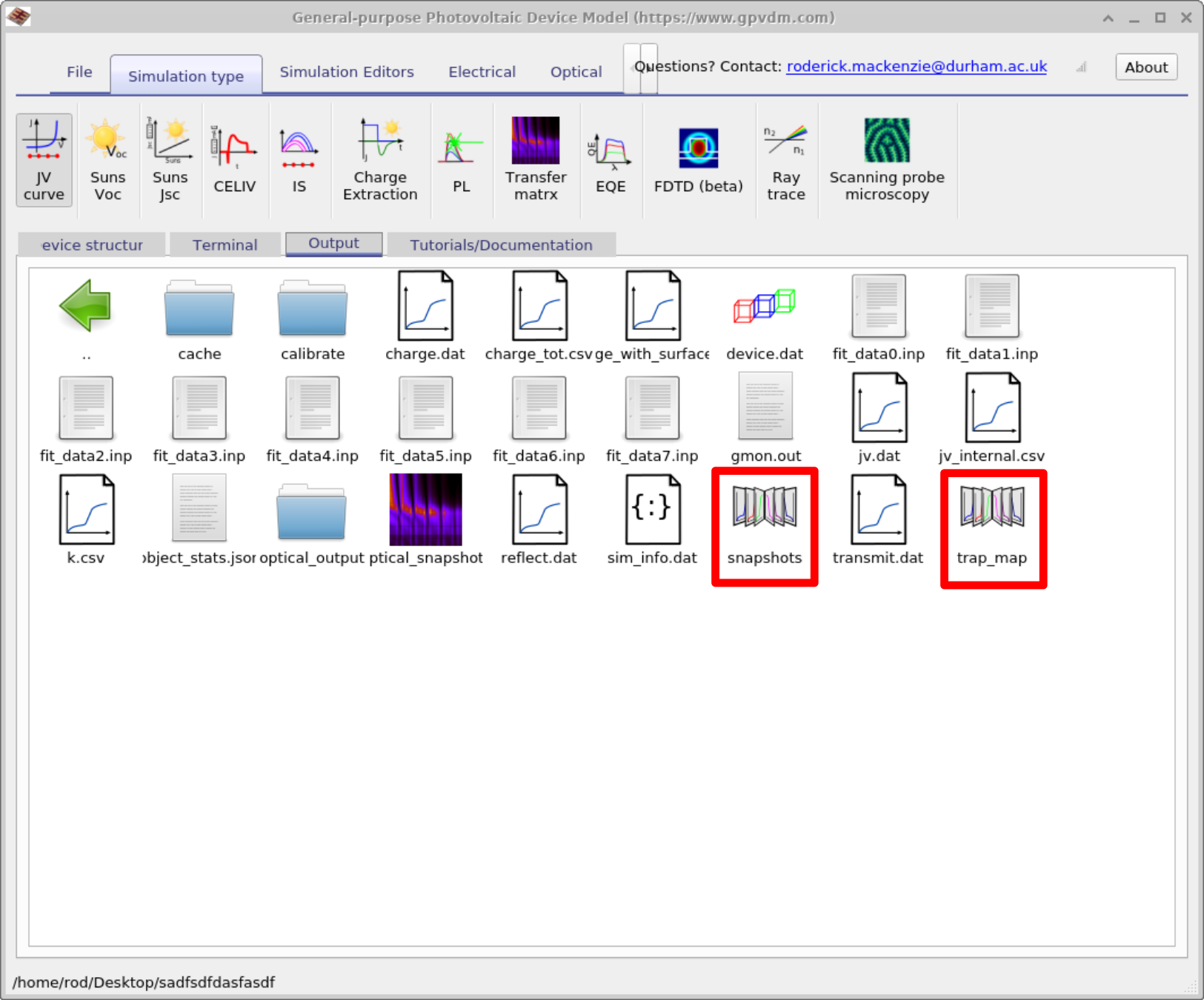
Sometimes it is advantageous to disable snapshots if you are not interested in the intermediate output because writing snapshots can significantly increase disk I/O and simulation runtime. Conversely, enabling snapshots can provide extremely useful insight into the internal device physics.

The snapshot controls also allow you to reduce the output frequency. For example, rather than writing every timestep or every voltage point, the simulation can instead store every second, third, or fourth step depending on the level of detail required.

Viewing snapshots

If you double-click on a snapshot directory, OghmaNano launches the snapshot viewer. The snapshot viewer provides a slider bar allowing you to move through the simulation outputs sequentially.

Snapshots can store many different types of data including:

• Band structures
• Carrier densities
• Trap occupancy maps
• Electric fields
• Optical power density
• Current densities
• Temperature distributions

Multiple datasets can often be displayed simultaneously, allowing direct comparison between different physical quantities during the simulation.

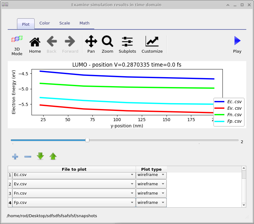
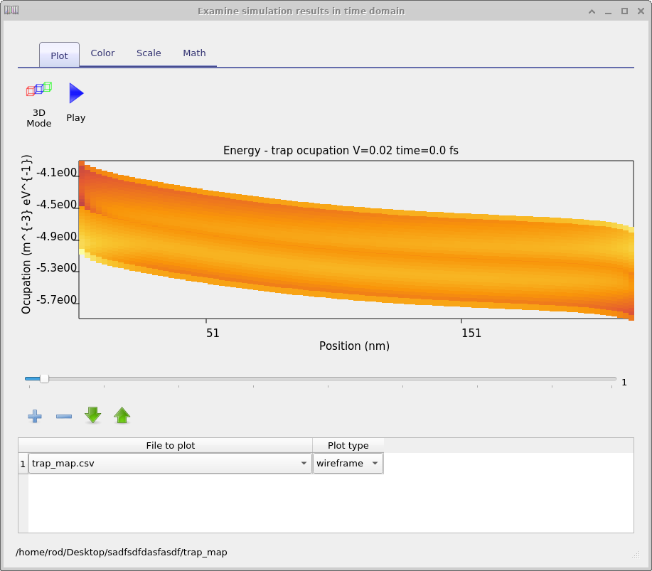
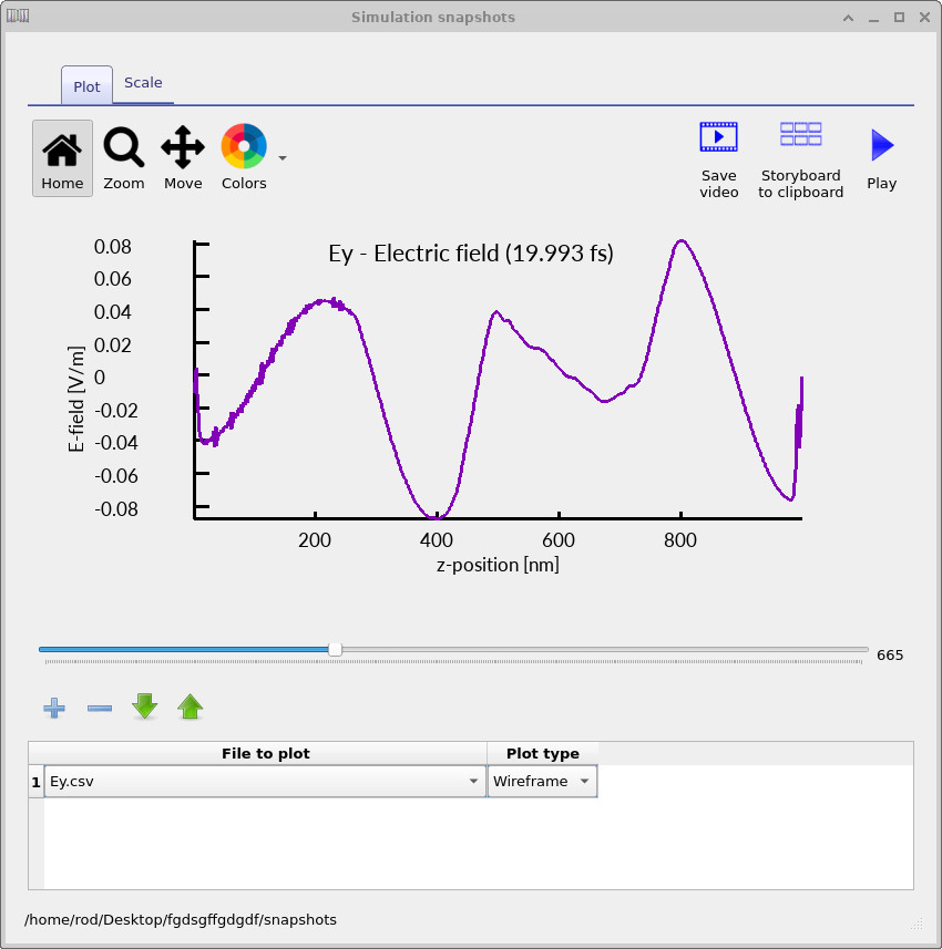
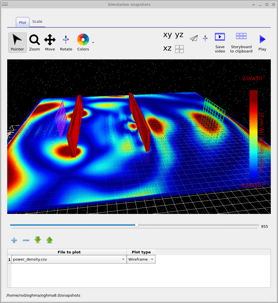
Internally, snapshots are simply collections of datasets written at different stages of the simulation. The viewer hides most of the underlying complexity and presents the outputs using a unified interface with playback controls, plotting options, scaling controls, and colour mapping.

How does the snapshot directory work?

Although the snapshot viewer presents a simplified interface, the underlying directory structure is actually very straightforward.

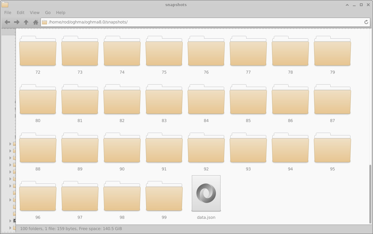
If you open the snapshot directory directly in the operating system file browser, as shown in ??, you will see that the directory simply contains a large number of numbered folders.

Each numbered folder corresponds to a particular simulation state:

• A voltage point in a JV simulation.
• A timestep in a transient simulation.
• A frame in an FDTD simulation.

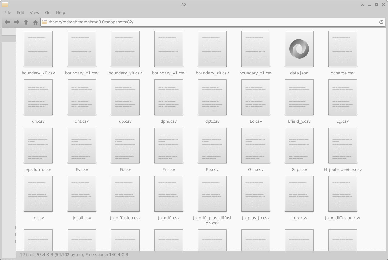
Inside each folder are the datasets associated with that particular simulation state. For electrical simulations these may include quantities such as:

• Conduction band energy (Ec.csv)
• Valence band energy (Ev.csv)
• Quasi-Fermi levels (Fn.csv, Fp.csv)
• Carrier densities
• Current densities
• Electric fields
• Recombination rates

Snapshots can be written either in human-readable CSV format or compact binary format, exactly as described in Understanding Output Files in OghmaNano.

In general, snapshots provide one of the most powerful ways to understand what is physically occurring inside a simulation because they expose the internal state of the device as the solver evolves toward the final solution.