Excited states in emissive materials
1. Introduction
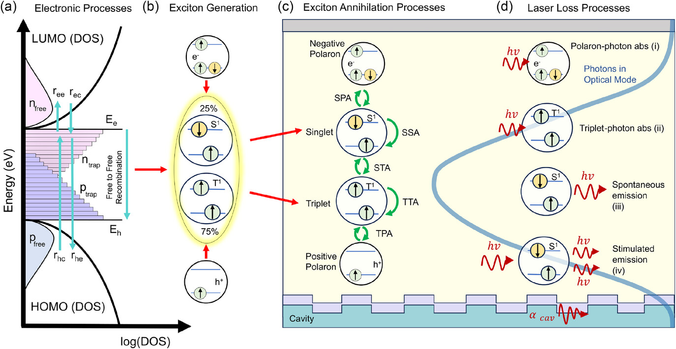
In LEDs and OLEDs, light emission does not occur directly from free charge carriers but from excited states (excitons) formed when electrons and holes recombine. These excited states exist as singlets and triplets, each with different decay pathways, interaction mechanisms, and radiative efficiencies. The balance between their formation, conversion, and loss processes ultimately determines the brightness, efficiency, and roll-off behaviour of the device. Consequently, a realistic model must explicitly track the populations of these excited states. Since excitons are generated by carrier recombination, this requires coupling to a drift–diffusion description of charge transport, which provides the local carrier densities and recombination rates that act as the pumping terms for the excited-state system.
In practice, this means solving the drift–diffusion equations together with a set of coupled rate equations describing singlet and triplet populations, and, where relevant, photon or optical mode dynamics. The exact combination of equations depends on the problem being studied: for example, modelling OLED efficiency may require only exciton rate equations, whereas modelling organic lasers additionally requires coupling to photon populations and cavity effects. The level of detail included can therefore be adjusted depending on whether a minimal or more complete physical description of the device is required.
💡 Note: For most OLED simulations, it is not necessary to include excited states. This is an advanced feature and is primarily important when modelling efficiency roll-off at high current densities, where exciton–exciton and exciton–polaron interactions become significant.
2. Overview
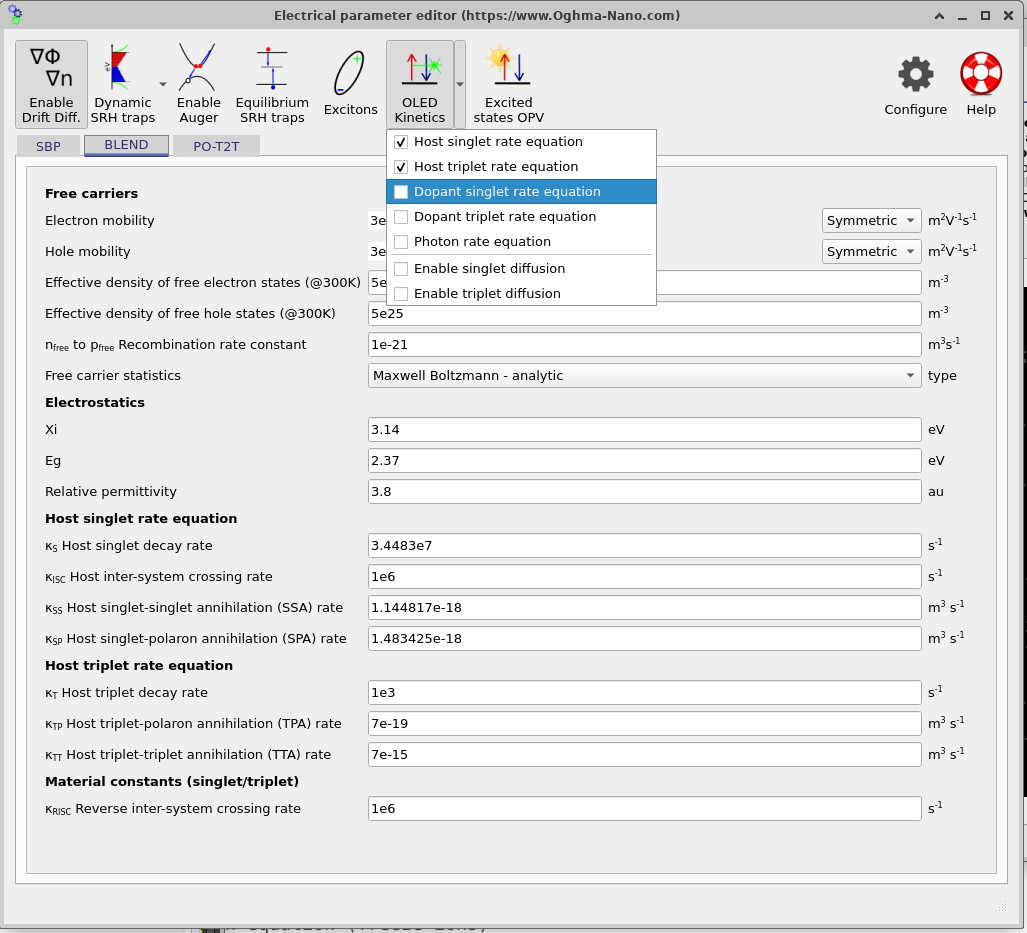
OghmaNano can solve up to four coupled singlet and triplet rate equations on top of the drift-diffusion equations in 1D, as illustrated schematically in ??. These are the singlet equation in the host, the triplet equation in the host, the singlet equation in the dopant, and the triplet equation in the dopant. The model can be enabled by first depressing the OLED kinetics button and then selecting which equations are required from the drop-down menu, as shown in ??. For most OLED simulations, only the first two equations, corresponding to the host singlet and host triplet populations, are normally required. A photon rate equation is also available for users who wish to simulate laser operation. These equations are discussed in detail below.
This model has been published in the following papers, where you can read more about its application to experimental data: A. Bickerdike et al. Unravelling the Spatiotemporal Exciton Dynamics in Electrically Pumped Organic Laser Diodes and A. Bickerdike et al. Reverse Intersystem Crossing and Exciton Harvesting: A Pathway to Low Threshold in Multi-Resonant TADF Electrically Pumped Organic Semiconductor Lasers
3. Drift–diffusion equations
Before solving the excited-state rate equations, it is first necessary to determine how charge carriers are injected, transported, and recombine within the device. This is done using the drift–diffusion equations, which provide the electron and hole densities and the recombination rates that act as the pumping terms for the excited-state system. These are the standard drift–diffusion equations used to describe charge transport in semiconductors, including carrier drift in the electric field, diffusion due to concentration gradients, and bimolecular recombination. A full description of these equations can be found here: Drift–diffusion theory, and a detailed derivation here: Derivation of the drift–diffusion equations.
In these equations, \(n\) and \(p\) are the electron and hole densities, \(\mathbf{J}_n\) and \(\mathbf{J}_p\) are the corresponding current densities, \(\mu_n\) and \(\mu_p\) are the mobilities, \(D_n\) and \(D_p\) are the diffusion coefficients, \(\phi\) is the electrostatic potential, \(G_n\) and \(G_p\) are generation rates, \(R_{\mathrm{free}}\) is the bimolecular recombination rate with coefficient \(k_r\), and \(R_{\mathrm{trap}}\) is the trap-assisted recombination rate. The quantities \(n_0\) and \(p_0\) denote equilibrium carrier densities.
Electron continuity
\[ \frac{\partial n}{\partial t} = \frac{1}{q}\nabla \cdot \mathbf{J}_n \;-\; R_{\mathrm{free}} \;-\; R_{\mathrm{trap}} \;+\; G_n, \qquad \mathbf{J}_n = -\,q\mu_n n \nabla\phi \;+\; q D_n \nabla n \]
Hole continuity
\[ \frac{\partial p}{\partial t} = -\,\frac{1}{q}\nabla \cdot \mathbf{J}_p \;-\; R_{\mathrm{free}} \;-\; R_{\mathrm{trap}} \;+\; G_p, \qquad \mathbf{J}_p = \;q\mu_p p \nabla\phi \;-\; q D_p \nabla p \]
Singlet population (host)
\[ \frac{dN_S}{dt} = \frac{1}{4}\big(\gamma_{\mathrm{free}} R_{\mathrm{free}} + \gamma_{\mathrm{trap}} R_{\mathrm{trap}}\big) + \frac{1}{4}\kappa_{TT}N_T^{2} - (\kappa_{\mathrm{FRET}}P_{OD} + \kappa_S + \kappa_{ISC})N_S - \Big(\tfrac{7}{4}\kappa_{SS}N_S + \kappa_{SP}(n_{\mathrm{free}}+p_{\mathrm{free}}) + \kappa_{ST}N_T\Big)N_S \]
Triplet population (host)
\[ \frac{dN_T}{dt} = \frac{3}{4}\big(\gamma_{\mathrm{free}} R_{\mathrm{free}} + \gamma_{\mathrm{trap}} R_{\mathrm{trap}}\big) + \kappa_{ISC}N_S + \frac{3}{4}\kappa_{SS}N_S^{2} - (\kappa_{DEXT}P_{OD} + \kappa_T + \kappa_{TP}(n_{\mathrm{free}}+p_{\mathrm{free}}))N_T - \frac{5}{4}\kappa_{TT}N_T^{2} \]
Singlet population (dopant)
\[ \frac{dN_{SD}}{dt} = \kappa_{\mathrm{FRET}}P_{OD}N_S + \frac{1}{4}\kappa_{TTD}N_{TD}^{2} - (\kappa_{SD} + \kappa_{ISCD})N_{SD} - \Big(\tfrac{7}{4}\kappa_{SSD}N_{SD} + \kappa_{SPD}(n_{\mathrm{free}}+p_{\mathrm{free}}) + \kappa_{STD}N_{TD}\Big)N_{SD} - \xi P_{HO}\big(N_{SD} - WN_{OD}\big) \]
Triplet population (dopant)
\[ \frac{dN_{TD}}{dt} = \kappa_{DEXT}P_{OD}N_T + \kappa_{ISCD}N_{SD} + \frac{3}{4}\kappa_{SSD}N_{SD}^{2} - \kappa_{TD}N_{TD} - \frac{5}{4}\kappa_{TTD}N_{TD}^{2} - \kappa_{TPD}N_{TD}(n_{\mathrm{free}}+p_{\mathrm{free}}) \]
Photon population (optical mode)
\[ \frac{dP_{HO}}{dt} = \beta_{sp}\kappa_{SD}N_{SD} + \big(\Gamma \xi (N_{SD} - WN_{OD}) - \kappa_{CAV}\big) P_{HO} \]
Dopant population constraint
\[ N_{OD} = N_{DOP} - N_{SD} - N_{TD} \]
💡 Note: The host singlet and triplet equations can also include diffusion terms, which can be enabled from the drop-down menu at the top of the electrical editor. However, these are typically kept disabled, as they make the system more difficult to solve numerically, increasing runtime and reducing solver robustness. In most cases this is not required, since excitons generally have short diffusion lengths, so enabling diffusion provides limited benefit unless specifically needed.
4. Light emission
Light emission in the model arises from carrier recombination and/or exciton relaxation processes. This emitted light feeds directly into the calculated quantum efficiency outputs, including external quantum efficiency (EQE), light–voltage (L–V) curves, light–current (L–I) curves, and the emissive spectrum of the material. The point at which light is extracted from the model depends on which physical processes are enabled. If the excitonic model is disabled, emission is taken directly from the recombination terms (\(R_{\mathrm{free}}\) and \(R_{\mathrm{trap}}\)). As progressively more equations are enabled, the emission is instead taken from the corresponding excitonic or optical populations. The specific emission pathways used under different model configurations are summarised below.
There are four ways that light can be emitted in the model, depending on which equations are enabled.
- When the singlet and triplet model is turned off, light is emitted directly from free carrier recombination; this also includes recombination via trap states, which can be written as \(R_{\mathrm{trap}}\); this contribution can be enabled or disabled independently.
- If the singlet and triplet equations are enabled, emission is taken from singlet decay.
- If the host–dopant equations are enabled, emission is taken from the dopant singlet population.
- If the photon rate equation is enabled, emission is taken from the cavity loss term.
| Model configuration | Emission source | Photon generation rate |
|---|---|---|
| No exciton model | Free carrier recombination | \(G_\gamma = \eta_{\mathrm{ph}}\left(R_{\mathrm{free}} + R_{\mathrm{trap}}\right)\) |
| Singlet/triplet enabled | Host singlet decay | \(G_\gamma = \eta_{\mathrm{ph}}\,\kappa_S N_S\) |
| Singlet/triplet + dopant enabled | Dopant singlet decay | \(G_\gamma = \eta_{\mathrm{ph}}\,\kappa_{SD} N_{SD}\) |
| Photon rate equation enabled | Cavity loss | \(G_\gamma = \kappa_{\mathrm{CAV}} P_{HO}\) |
5. Outputs
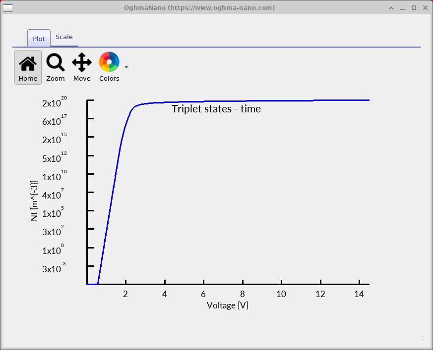
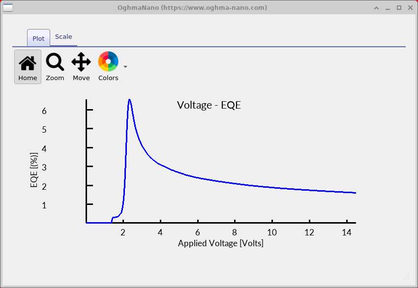
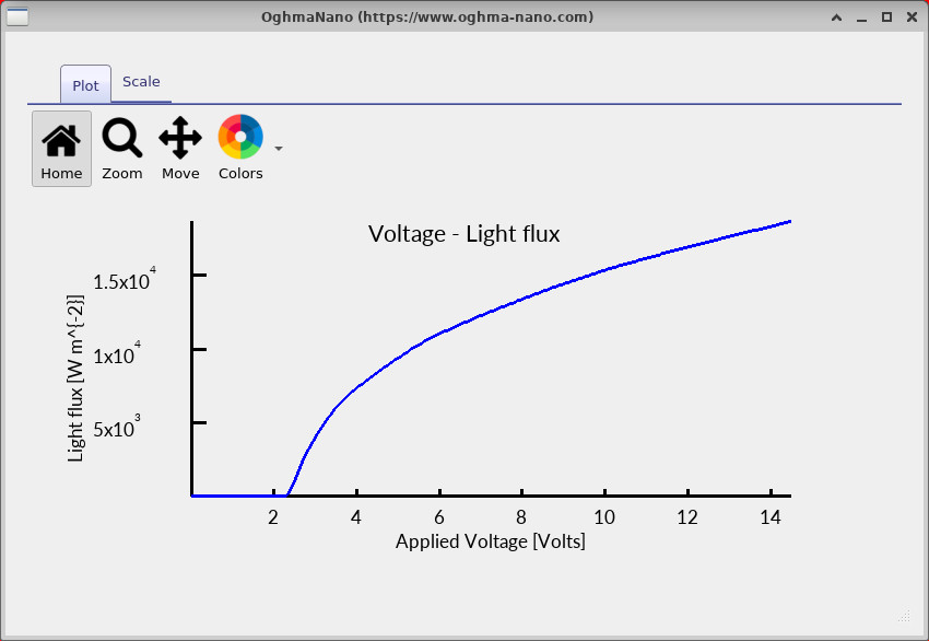
The excited-state model produces a range of additional outputs that can be used to analyse the behaviour of OLED and laser structures. Spatial snapshots of the singlet and triplet populations can be viewed from the snapshots directory, as shown in ??. In this example, the files EX_Ns.csv and EX_Nt.csv are plotted as a function of position, corresponding to the singlet and triplet densities respectively. Time- or voltage-dependent sweep outputs can also be generated, as illustrated in ??, where the triplet density is plotted as a function of applied voltage. The effect of the excited-state model is also reflected in the calculated device performance metrics. For example, the EQE curve shown in ?? drops at higher voltage due to singlet-triplet annihilation. Likewise, the light-voltage curve shown in ?? includes the effect of the singlet-triplet equations through the way light is coupled out of the model.
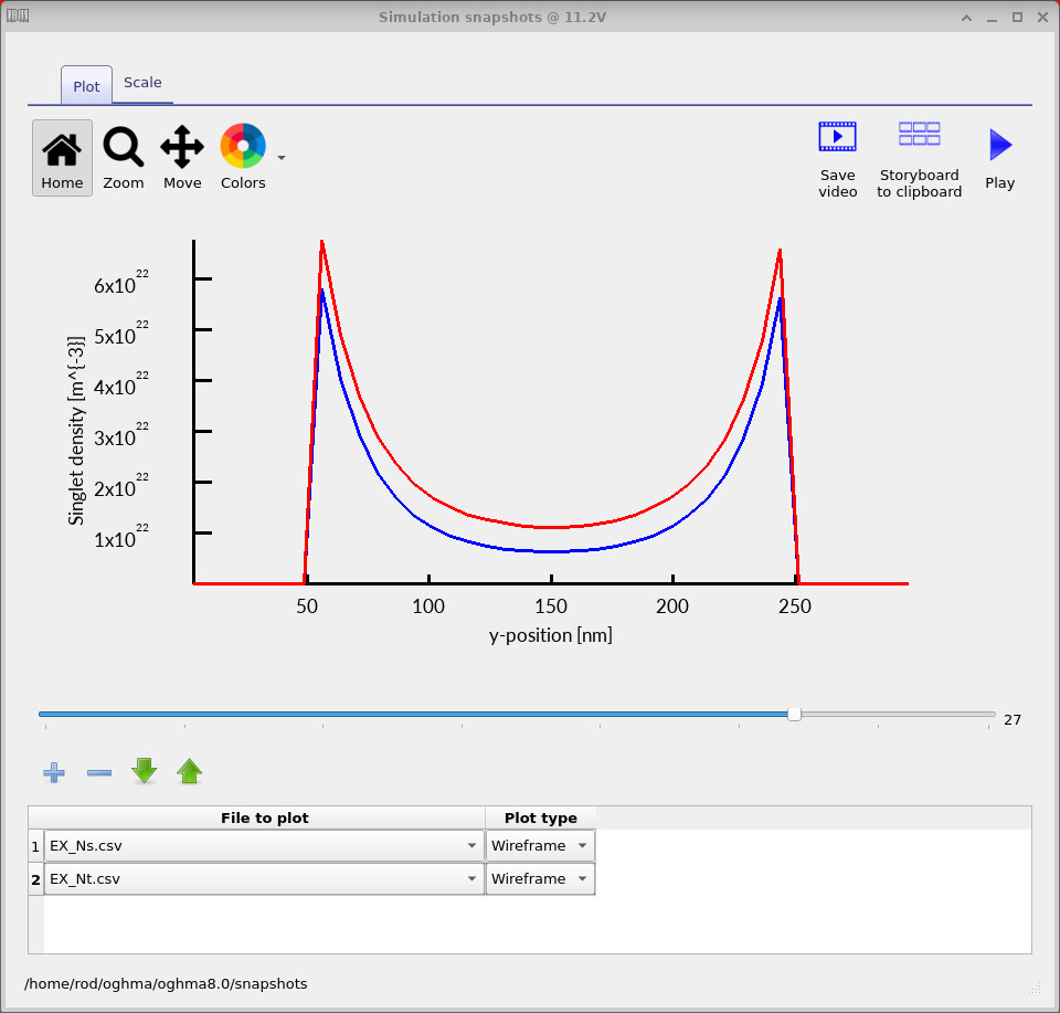
EX_Ns.csv and EX_Nt.csv, corresponding to the singlet and triplet densities plotted as a function of position.
6. Variables and constants
State variables
| Symbol | Description |
|---|---|
| \(N_S\) | Singlet population (host). |
| \(N_T\) | Triplet population (host). |
| \(N_{SD}\) | Singlet population (dopant). |
| \(N_{TD}\) | Triplet population (dopant). |
| \(P_{HO}\) | Photon population (optical mode). |
| \(N_{OD}\) | Ground-state dopant population. |
| \(N_P\) | Polaron population. |
Kinetic coefficients (host)
| Symbol | Description | JSON token |
|---|---|---|
| \(\kappa_S\) | Singlet population (host) decay rate. | singlet_k_s |
| \(\kappa_{ISC}\) | Inter-system crossing rate from singlet (host) to triplet (host). | singlet_k_isc |
| \(\kappa_{SS}\) | Singlet–singlet annihilation rate for singlet population (host). | singlet_k_ss |
| \(\kappa_{SP}\) | Singlet–polaron annihilation rate for singlet population (host). | singlet_k_sp |
| \(\kappa_{ST}\) | Singlet–triplet annihilation rate between singlet (host) and triplet (host). | singlet_k_st |
| \(\kappa_T\) | Triplet population (host) decay rate. | singlet_k_t |
| \(\kappa_{TP}\) | Triplet–polaron annihilation rate for triplet population (host). | singlet_k_tp |
| \(\kappa_{TT}\) | Triplet–triplet annihilation rate for triplet population (host). | singlet_k_tt |
Transfer coefficients (host → dopant)
| Symbol | Description | JSON token |
|---|---|---|
| \(\kappa_{\mathrm{FRET}}\) | Förster transfer rate from singlet population (host) to singlet population (dopant). | singlet_k_fret |
| \(\kappa_{DEXT}\) | Dexter transfer rate from triplet population (host) to triplet population (dopant). | singlet_k_dext |
Kinetic coefficients (dopant)
| Symbol | Description | JSON token |
|---|---|---|
| \(\kappa_{SD}\) | Singlet population (dopant) decay rate. | singlet_k_sd |
| \(\kappa_{ISCD}\) | Inter-system crossing rate from singlet (dopant) to triplet (dopant). | singlet_k_iscd |
| \(\kappa_{SPD}\) | Singlet–polaron annihilation rate for singlet population (dopant). | singlet_k_spd |
| \(\kappa_{STD}\) | Singlet–triplet annihilation rate between singlet (dopant) and triplet (dopant). | singlet_k_std |
| \(\kappa_{SSD}\) | Singlet–singlet annihilation rate for singlet population (dopant). | singlet_k_ssd |
| \(\kappa_{TD}\) | Triplet population (dopant) decay rate. | singlet_k_td |
| \(\kappa_{TTD}\) | Triplet–triplet annihilation rate for triplet population (dopant). | singlet_k_ttd |
| \(\kappa_{TPD}\) | Triplet–polaron annihilation rate for triplet population (dopant). | singlet_k_tpd |
Optical and cavity coefficients
| Symbol | Description | JSON token |
|---|---|---|
| \(\Gamma\) | Confinement factor scaling coupling between singlet population (dopant) and photon population. | singlet_gamma |
| \(W\) | Spectral overlap factor between photon population and ground-state dopant population. | singlet_W |
| \(\xi\) | Stimulated-emission coupling between singlet population (dopant) and photon population. | — |
| \(\kappa_{CAV}\) | Photon loss rate from the optical mode. | — |
| \(\beta_{sp}\) | Spontaneous emission coupling into the photon population. | — |
| \(\gamma\) | Polaron recombination coefficient generating singlet and triplet populations (host). | — |
Material and composition parameters
| JSON token | Symbol | Description |
|---|---|---|
singlet_C |
\(C\) | Dopant concentration parameter used to define the amount of dopant present in the emissive medium. |
| — | \(N_{DOP}\) | Total dopant population density. |
| — | \(P_{OD}\) | Available dopant fraction or occupancy factor entering host-to-dopant transfer terms. |
| — | \(n_0,\;p_0\) | Equilibrium electron and hole densities used in the free-to-free recombination expression. |
GUI and control tokens
| JSON token | Symbol | Description |
|---|---|---|
singlet_enabled |
— | Boolean switch enabling or disabling the excited-state model in the GUI and solver. |
text_singlet_ |
— | GUI label token used to insert the “Excited states” heading. |