FDTD tutorial: Integrated Photonics Ring Resonator
1. Overview: what you will simulate
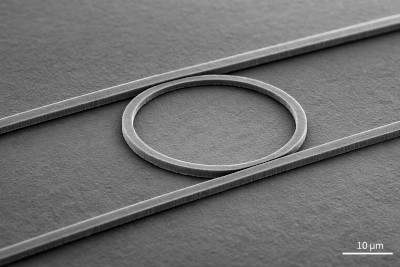
A photonic ring resonator is a compact optical cavity formed by a closed-loop waveguide placed next to one or more straight bus waveguides. Light launched into the bus can evanescently couple into the ring. When the optical path length of the ring satisfies the resonance condition (mλ = neffL), constructive interference builds up circulating power inside the cavity. Off-resonant wavelengths do not efficiently couple and instead remain in the bus waveguide.
Because of this wavelength-selective behaviour, ring resonators are widely used in photonic integrated circuits (PICs) for filtering, wavelength-division multiplexing (WDM), modulation, sensing, and on-chip signal routing. They are found in silicon photonics platforms for data communications, LiDAR systems, biosensors, and integrated optical signal processors. Their small footprint, CMOS compatibility, and strong field enhancement make them one of the fundamental building blocks of modern integrated photonics.
In this tutorial, we investigate a representative ring resonator structure (see ??) using the Finite-Difference Time-Domain (FDTD) method. We launch a guided mode into a straight waveguide, observe evanescent coupling into the ring, and monitor how optical power evolves in time.
The simulation allows you to:
- Visualise time-domain field evolution and power density snapshots,
- Observe energy build-up and decay inside the cavity,
- Measure transmitted and coupled power using time-domain detectors,
- Compare continuous-wave (CW) and pulsed excitation responses.
From a numerical perspective, this example exercises the full FDTD stack: geometry definition, source injection, perfectly matched layer (CPML) absorbing boundaries, time stepping, and detector extraction. Physically, it provides intuition for resonance, coupling strength, and cavity lifetime in integrated photonic devices.
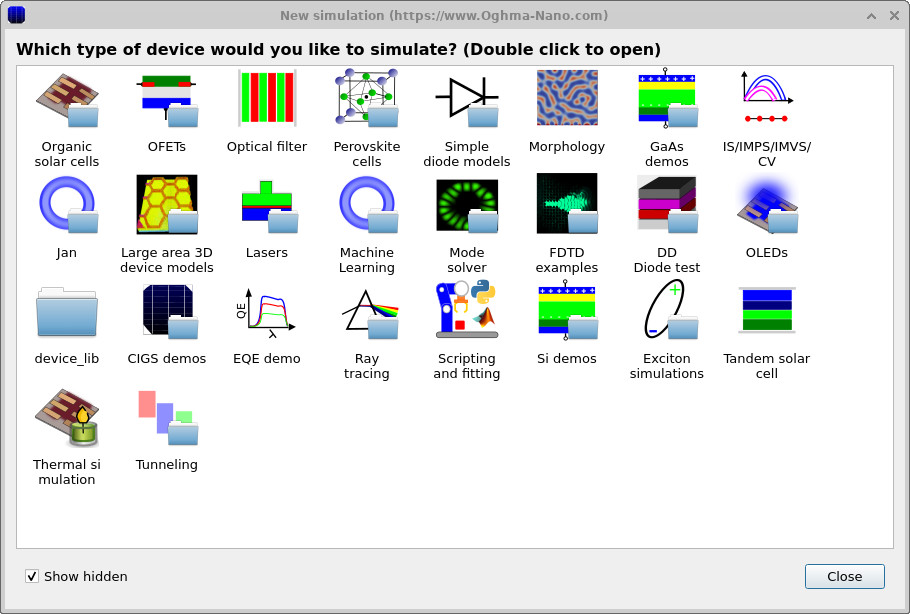
2. Making a new simulation
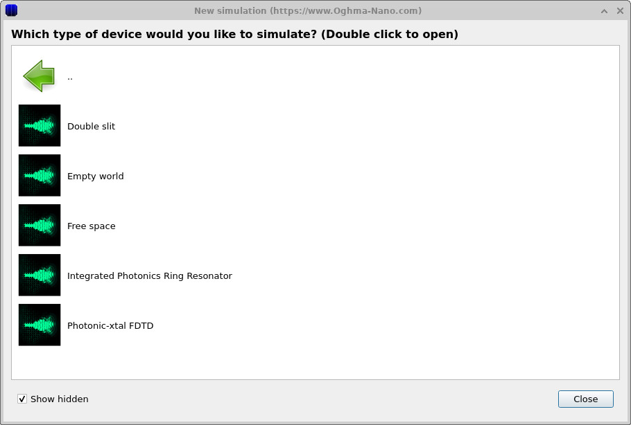
Open the New simulation window and select the FDTD examples category (??). Then choose the Integrated Photonics Ring Resonator example (??). This loads the main interface shown in ??.
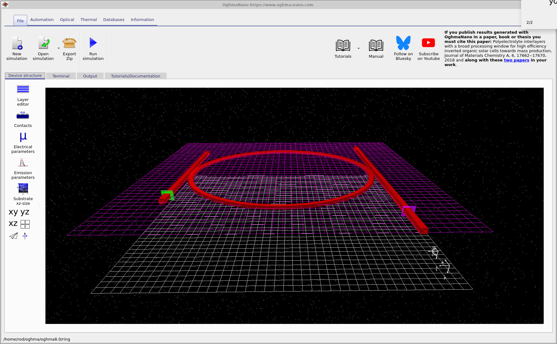
3. Orienting yourself in the main window
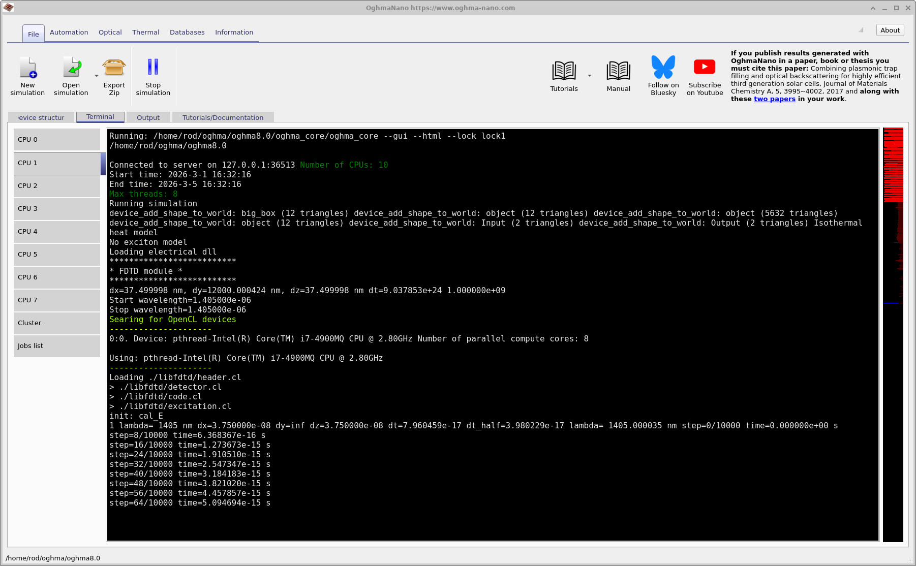
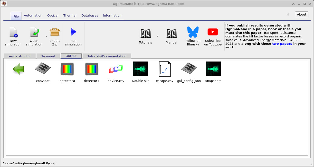
The device appears in the 3D view in the Device structure tab (??). The Terminal tab streams solver output during execution, and the Output tab lists the files produced by the simulation (snapshots, detectors, and configuration exports).
For this example you will mainly use:
- Run simulation (▶) to start the FDTD calculation.
- Terminal tab to confirm grid spacing, timestep, wavelength range, and OpenCL device selection.
- Output tab to open snapshots and detector files.
4. Running the simulation
snapshots/ folder and detector outputs from here.
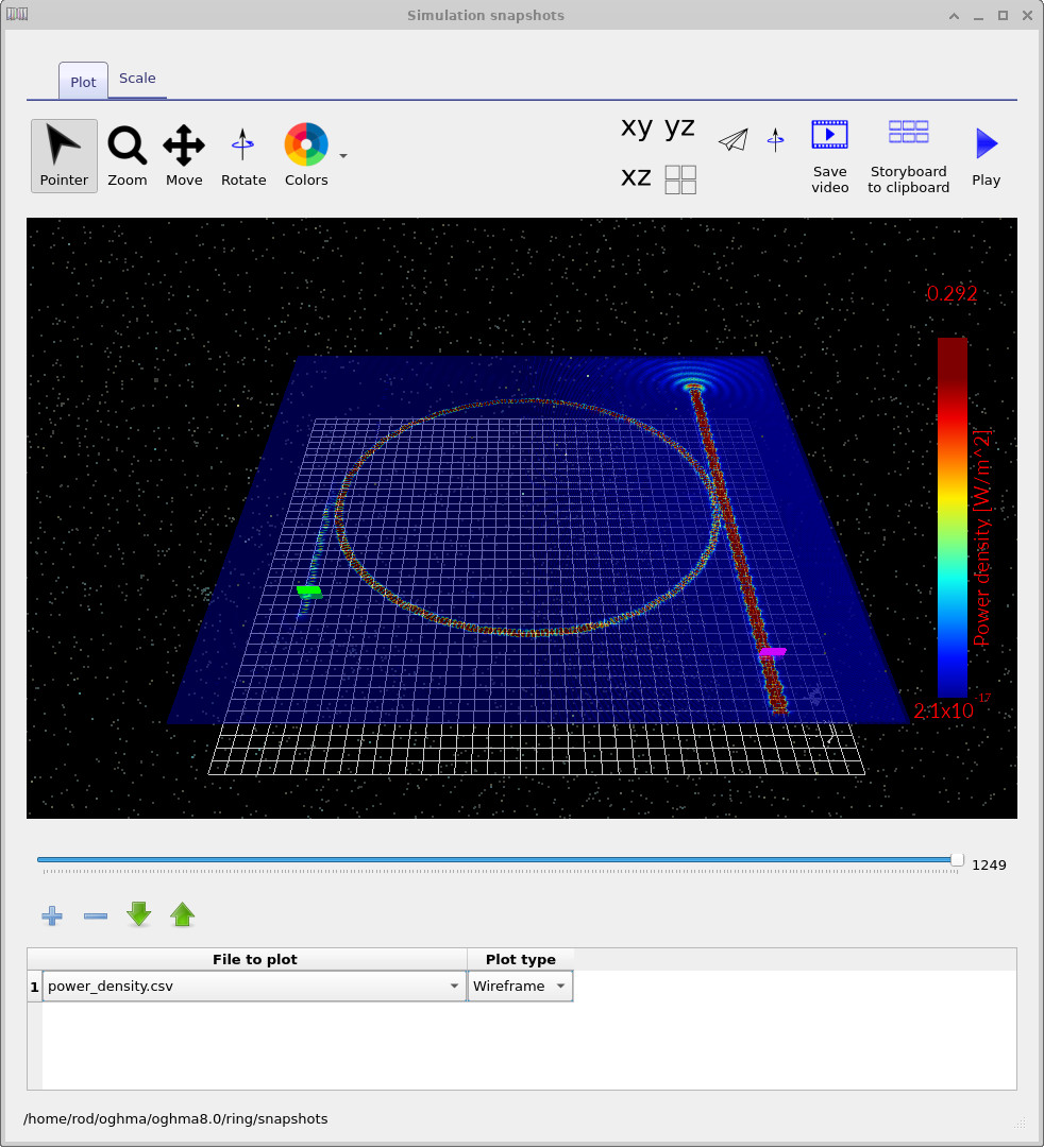
5. Viewing power density snapshots
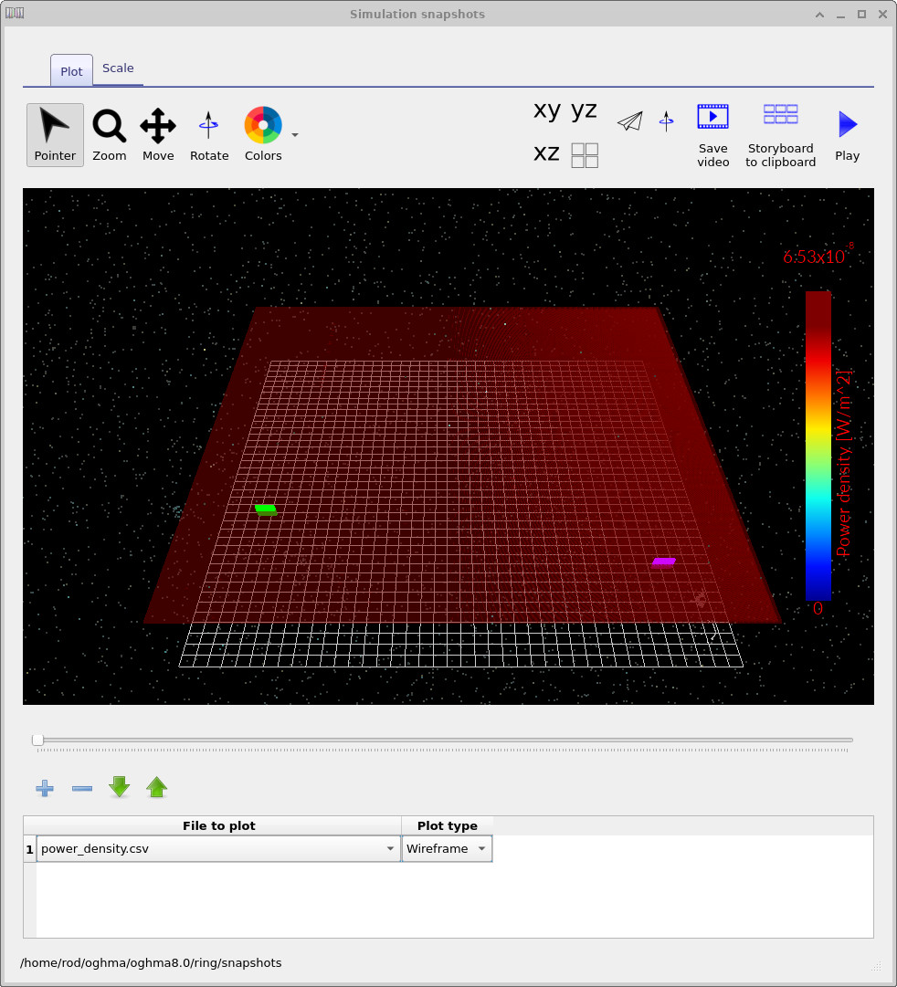
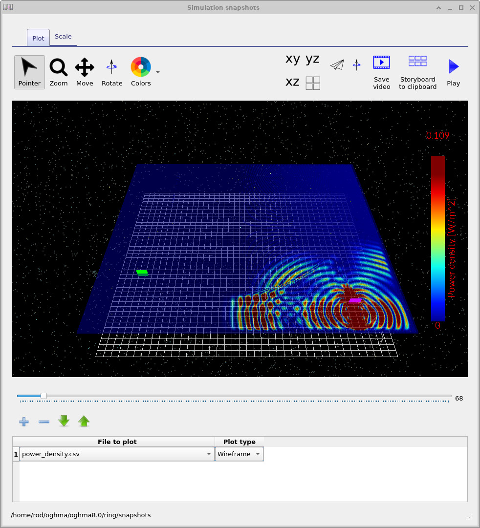
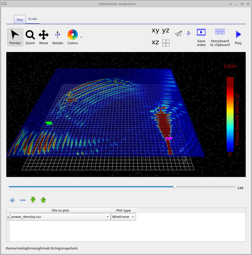
Open the snapshots/ output directory (from the Output tab) to launch the snapshot viewer. Plot
the power density file (for example power_density.csv) and use the slider to step through time.
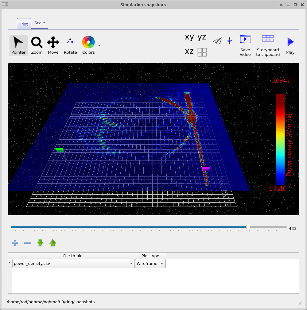
Representative snapshots are shown in
??–
??.
As the source launches into the bus waveguide, you should see energy propagating toward the coupling region, then coupling into the ring. Later snapshots show circulation and build-up in the ring, followed by steady routing to the output waveguide.


6. Viewing detector outputs
This example includes two detectors placed on the output waveguides. Open each detector file from the Output tab (see ??) and plot the recorded signal versus time. The two detector outputs are shown in ?? and ??.
In steady CW operation, you should expect the detector traces to approach a constant value after an initial transient. If you see persistent beating or a drifting baseline, it usually indicates either (i) a broadband excitation (not truly single-frequency), (ii) reflections from boundaries/ports, or (iii) an under-resolved geometry introducing dispersion.
7. Editing the light source: CW vs pulsed excitation
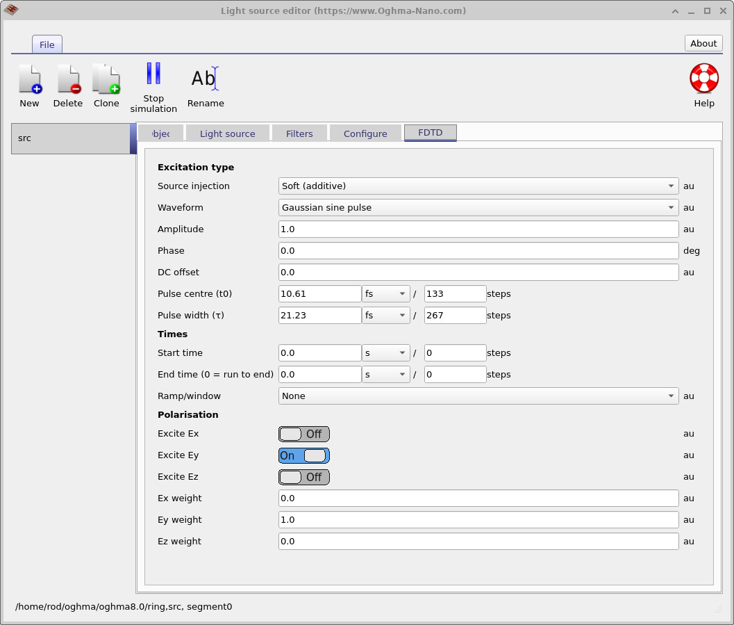
Open the light source editor for the simulation and locate the excitation waveform settings (??). Switch from a CW/gaussian-sine style excitation to a pulsed waveform (??). Then rerun the simulation and compare the detector outputs.
With pulsed excitation, the detector time series should show a clear transient response: an initial rise as energy couples into the ring, followed by a decay once the pulse has passed and the stored energy leaves via coupling and loss. If you want a single-number summary of “how resonant” the device is, measure the decay constant in the detector trace after the pulse peak; it is a direct proxy for the effective cavity lifetime in this configuration.
8. Quick checks and common failure modes
- No signal at detectors: check the source orientation/polarisation and that detectors are placed on guided regions, not in PML.
- Strong spurious radiation: check grid resolution at material boundaries and verify subpixel smoothing/averaging settings if enabled.
- Unstable growth: timestep too large (CFL). Reduce
dtor increase spatial resolution consistently. - Unexpected reflections: verify port termination, PML thickness, and that sources/detectors are not too close to boundaries.
👉 Next step: Once you are happy with the detector behaviour, the natural extension is a wavelength sweep (or a short broadband pulse + FFT) to extract the resonance spectrum and estimate \(Q\) from linewidth.
6. Viewing detector outputs
After the run completes, open the Output tab and locate power.csv
(??).
Double-clicking this file opens the detector power viewer for the selected detector.
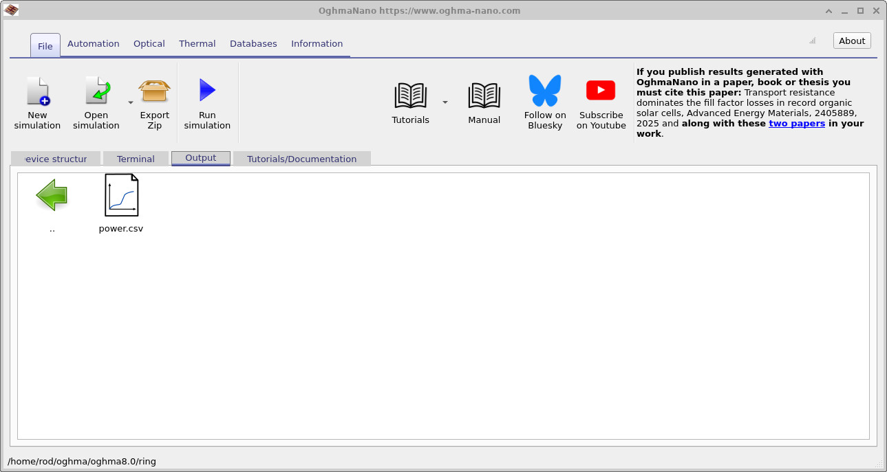
power.csv, which opens the detector power viewer.
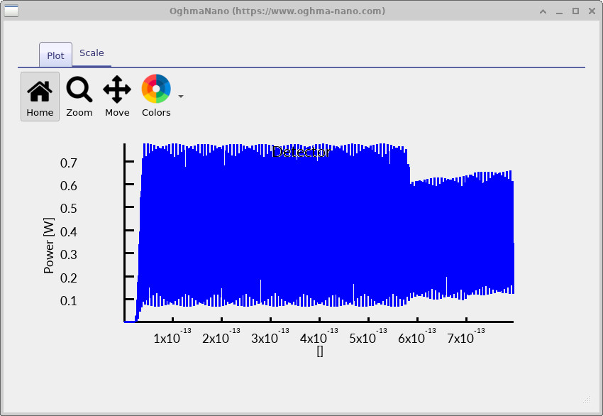
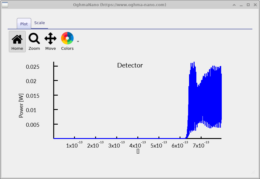
Compare ?? and ??. The near detector responds earlier, while the downstream detector responds later because the field must propagate through the bus/ring coupling region and then reach the monitored port.
7. Switching the excitation to a pulse
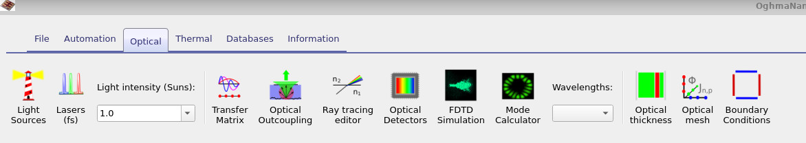
The source parameters are edited from the Optical ribbon (??). Click Light Sources to open the light source editor, shown in ??.
In the light source editor, open the FDTD tab and set the waveform to Gaussian sine pulse. This replaces continuous-wave excitation with a short pulse containing a carrier, allowing you to see transit delay and resonator build-up more clearly.
Rerun the simulation and then reopen the detector plots (??, ??). With a pulse, the detector signals typically show a clearer onset, a finite delay between ports, and a decay/ring-down that reflects loss and coupling strength.