Perovskite Solar Cell Tutorial – Simulating EQE
1. Introduction
External Quantum Efficiency (EQE) describes how efficiently a solar cell converts incident photons at each wavelength into collected charge carriers. In other words, it is the probability that a photon of a given energy contributes to the photocurrent. Experimentally, it is one of the most widely used characterization techniques for solar cells and provides detailed information about absorption, charge collection, and losses across the solar spectrum.
For perovskite devices, EQE is particularly helpful because the sharp absorption edge—and any extra optical loss—directly reflects material quality, whether the layers are the right thickness, and how light interferes within the stack. In this tutorial you will simulate EQE in OghmaNano, plot the spectrum, compare device stacks, and check your model against measured EQE.
2. Setting a simulation up for EQE
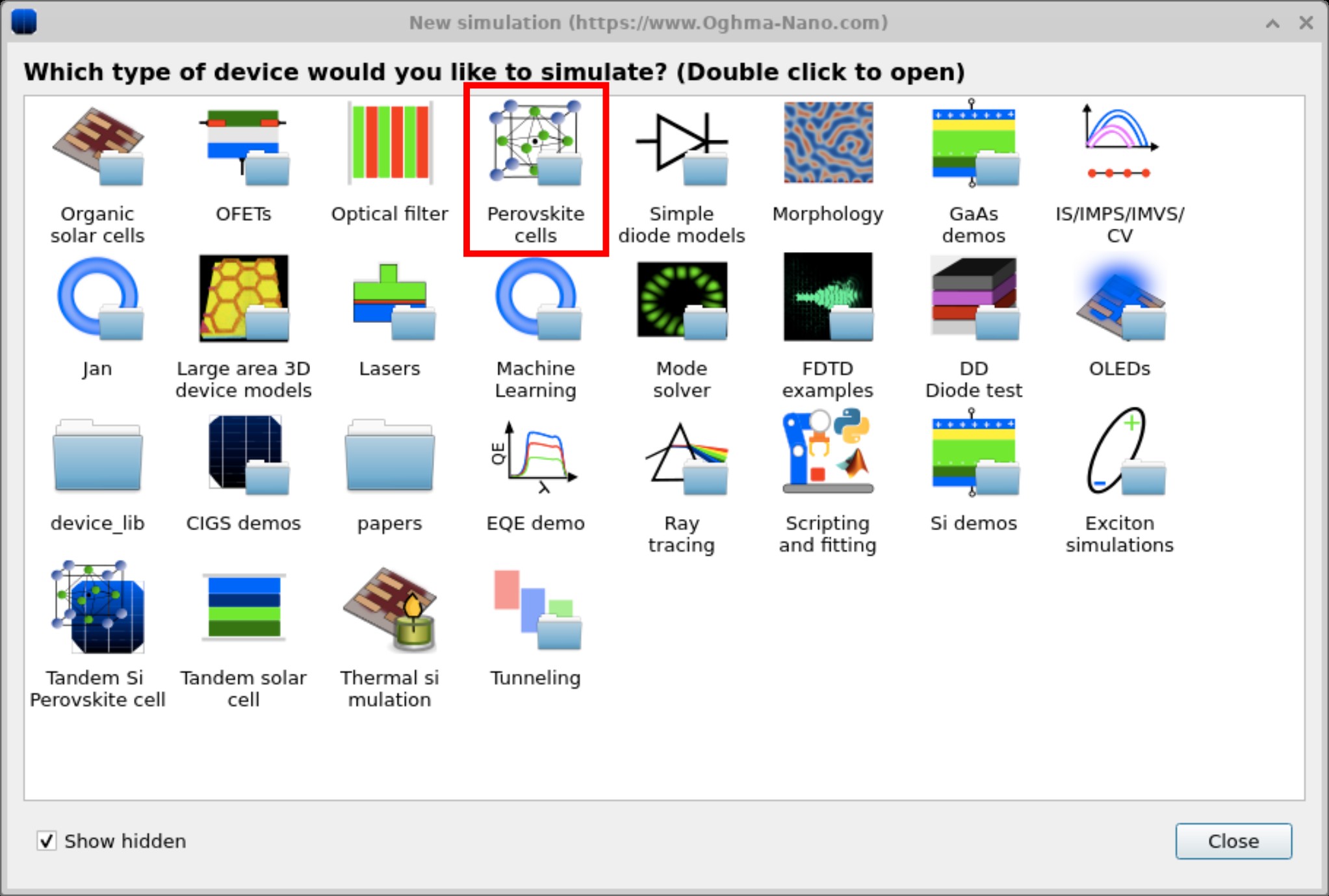
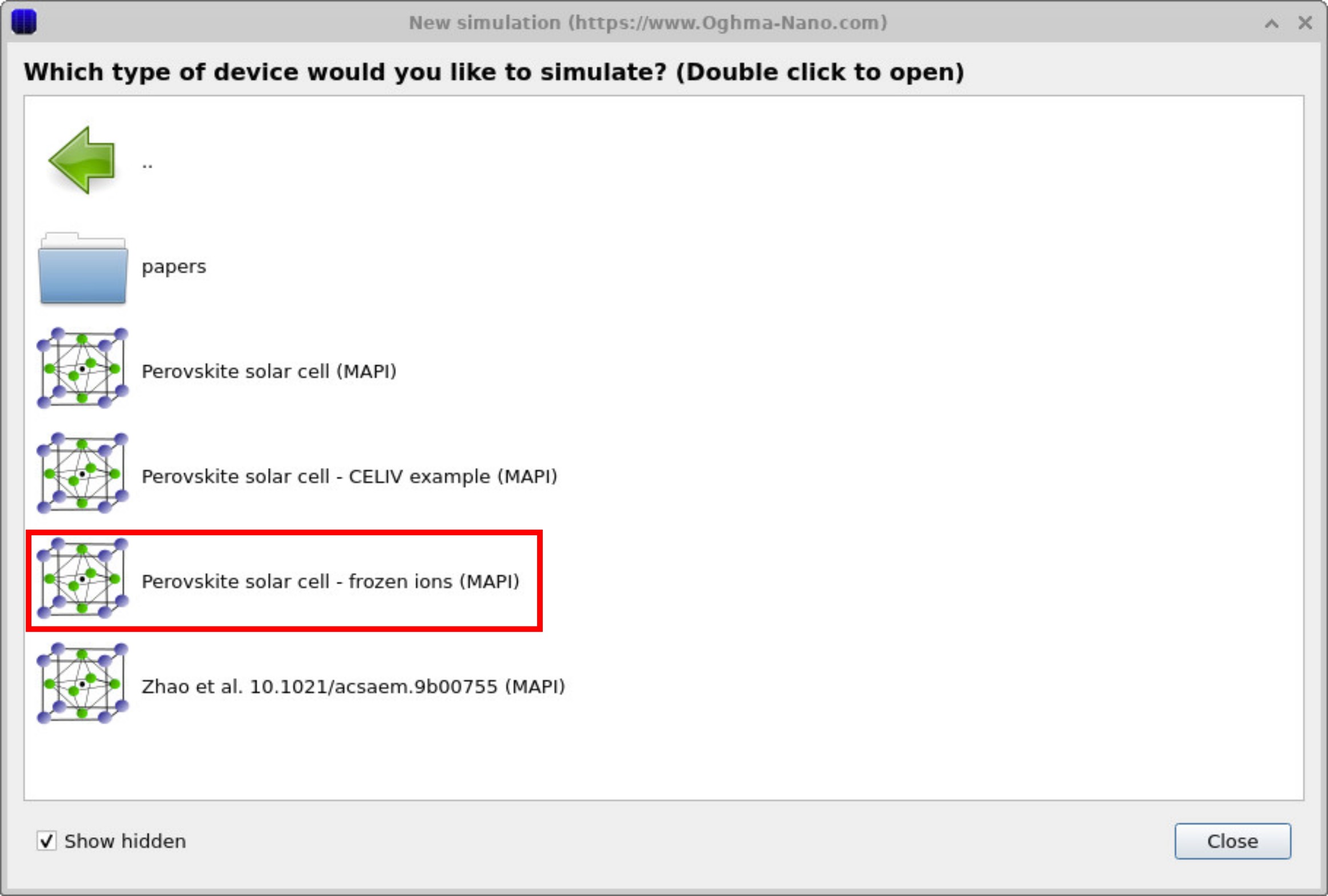
Start by launching OghmaNano. From the main window, click New simulation. The library of available device types appears as shown in ??. Double-click the Perovskite cells category to access example devices. Within the perovskite folder you will see a set of pre-built example simulations, such as MAPbI₃ devices and variants with ionic effects (frozen ions, CELIV, etc.). Select the Perovskite solar cell - frozen ions (MAPI) example, as shown in ??
💡 Tip: Make sure you select Perovskite solar cell - frozen ions (MAPI) - The frozen ions bit is important and will be explained later.
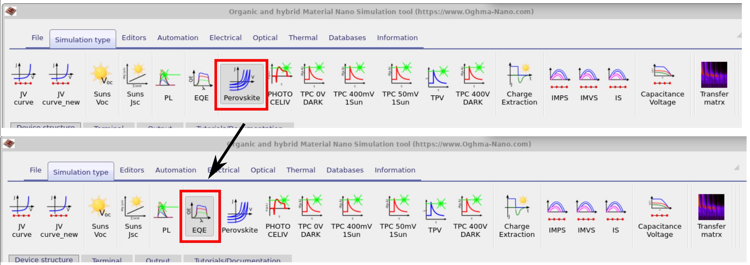
Before running the simulation, go to the Simulation type tab and switch from the default Perovskite hysteresis mode to EQE mode. This will set the simulation to be ready to perform EQE calculations.
3. Running the simulation
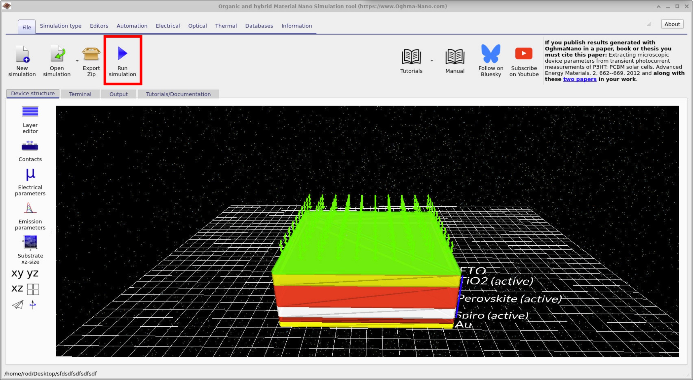
Once you have changed the simulation mode to EQE, go to the file tab. Press the Run simulation button (blue play icon) or press F9 to run the calculation. When the run is finished, go to the Output tab where you will see the files generated by the EQE simulation.
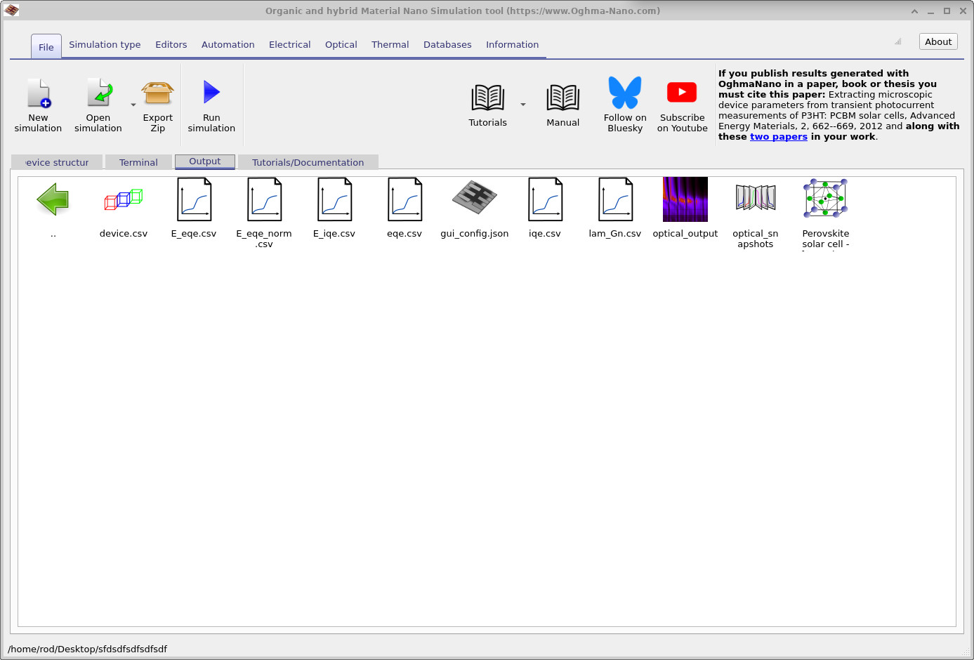
E_eqe.csv and E_iqe.csv for spectral analysis.
Once the simulation has finished, go to the Output tab. Double-click eqe.csv
to plot wavelength versus EQE (see
??).
If you double-click E_eqe.csv, you will see a plot of photon energy versus EQE (see
??).
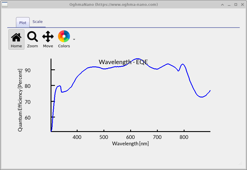
eqe.csv — plot of wavelength vs EQE.
This figure shows the EQE spectrum as a function of wavelength, as produced by the simulation.
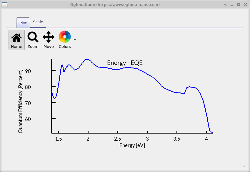
e_eqe.csv — plot of photon energy vs EQE.
This is the EQE spectrum expressed against energy (eV), also generated from the same run.
In principle, this is all you need to run EQE simulations. The same technique works for any device class (e.g., silicon or organic solar cells): simply click the EQE button, run the simulation, and the EQE spectrum will be produced. Because this tutorial uses a perovskite solar cell with mobile ions, there are a few extra details to consider. Read on if you want to understand the details.
4. Some more details
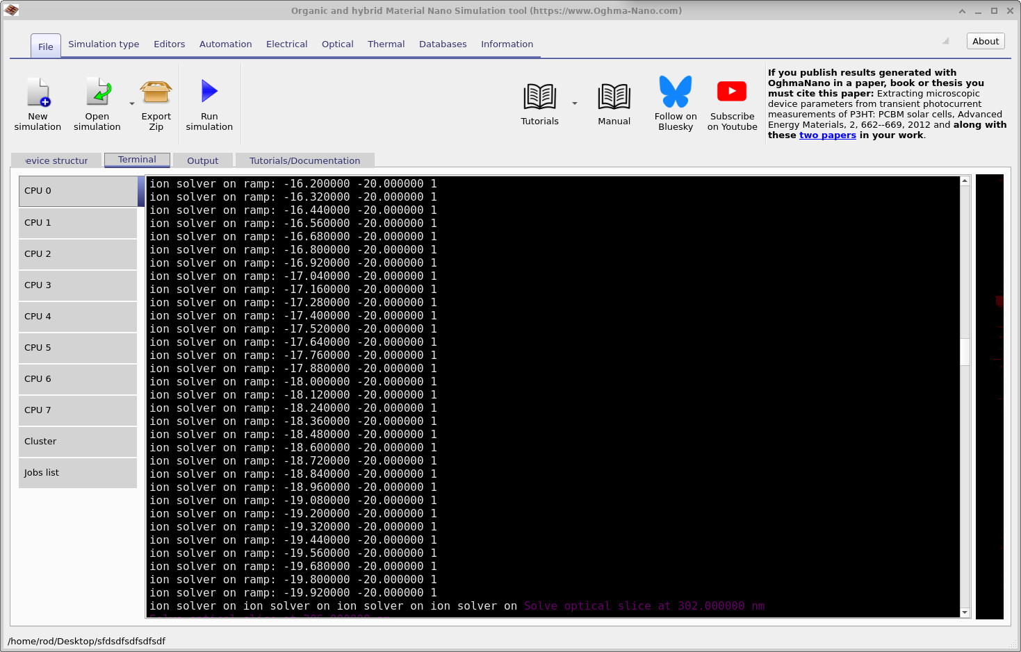
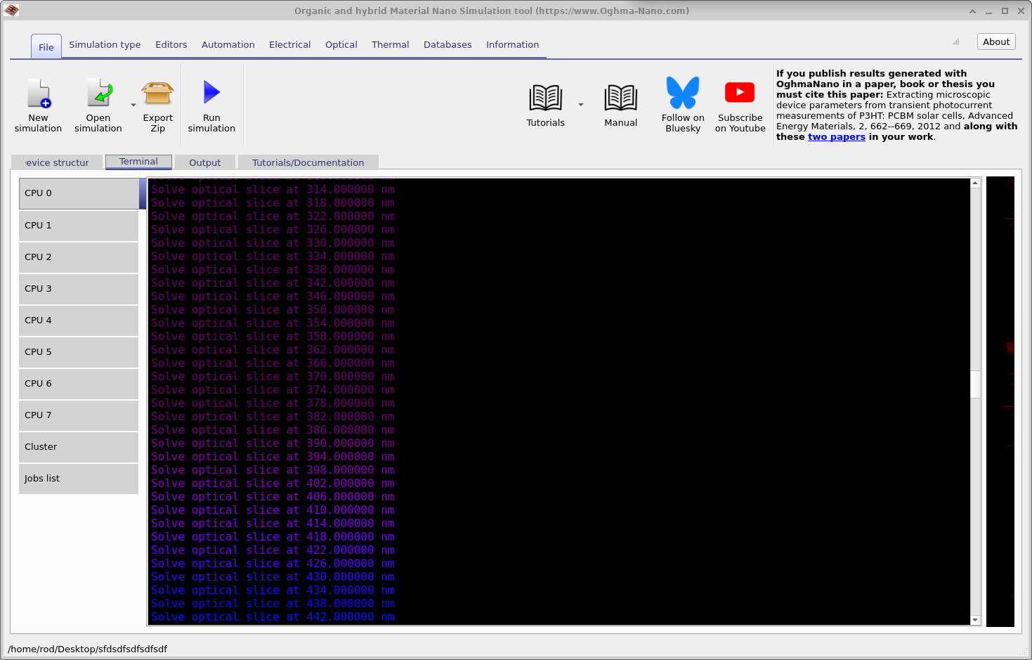
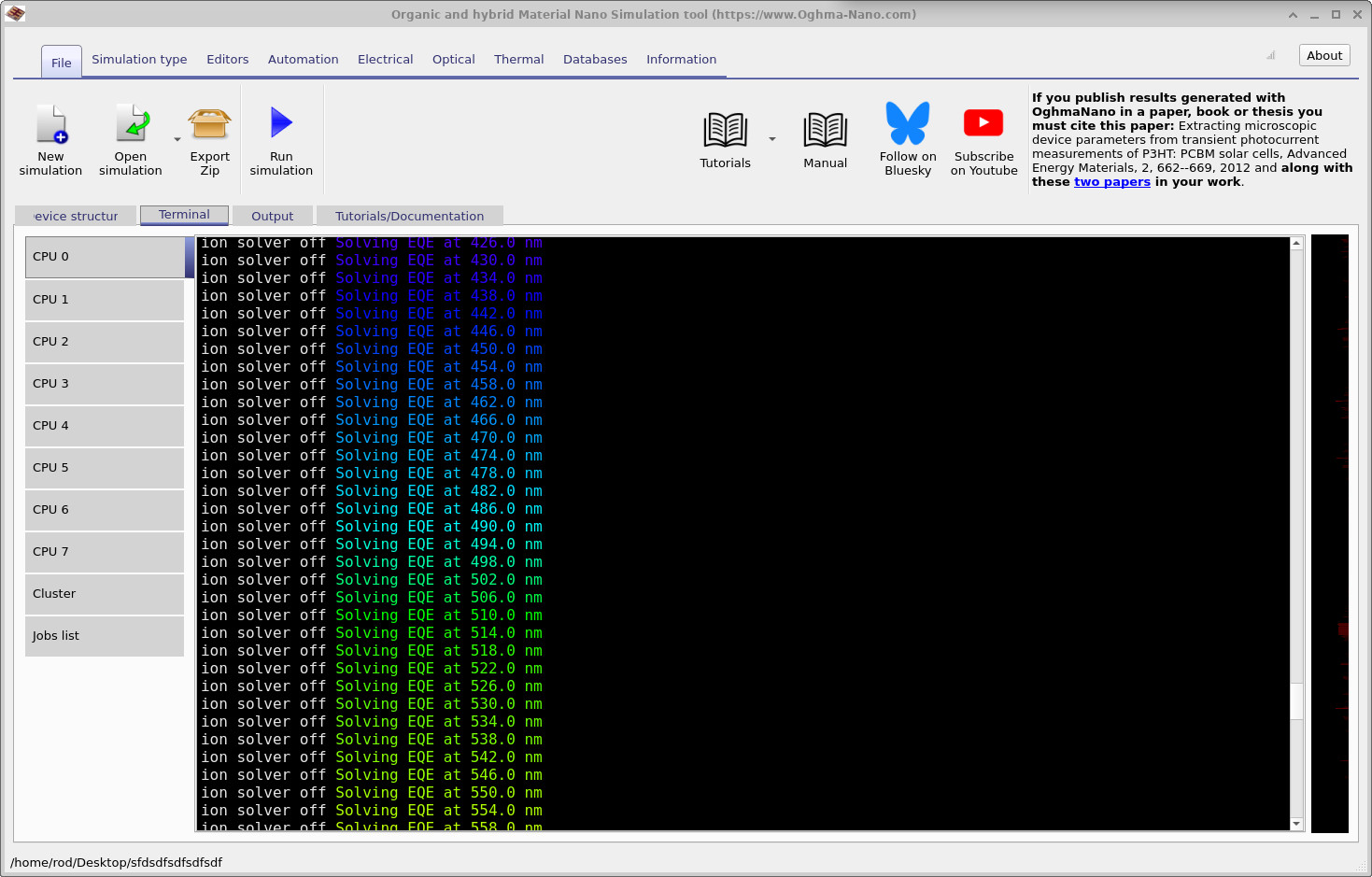
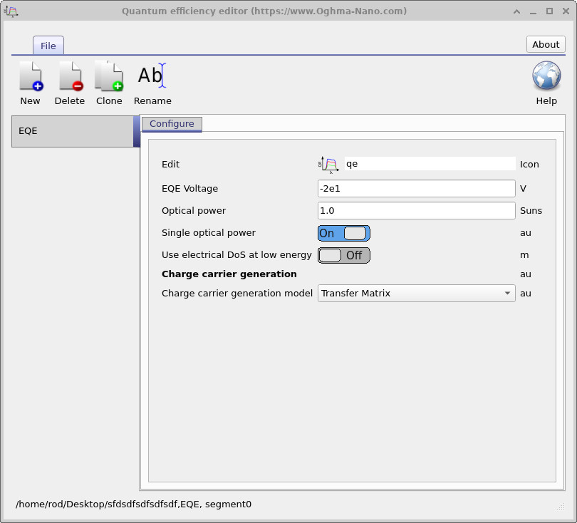
When you press the play button and run the EQE solver, it proceeds in three steps. Step 1: it ramps the device to the desired reverse-bias voltage at which EQE will be measured; (You can set this voltage through the EQE editor: Main window → Editors → EQE → EQE Voltage); Step 2: it runs the optical solver over the wavelength range of interest to compute the in-device photon distribution (see ??). Step 3: it performs the EQE calculation itself using those optical results at the target bias (see ??). You can see these different phases of the computation when you run the solver.
The voltage at which the EQE simulation is run can be set in the EQE Editor (see ??). Here the EQE Voltage parameter defines the bias used for the calculation, and the editor is accessed from the Editors ribbon in the main window. The advantage of running EQE at a more negative voltage is that you minimise the effect of carrier recombination. The closer you get to zero volts, and especially if you enter forward bias, the simulation will include increasing amounts of recombination. In that regime, the result is no longer a clean measure of the intrinsic EQE.
5. EQE in perovskites
🔧 Advanced detail: The section below explains how OghmaNano uses Lua microcode to control the mobile-ion solver during EQE calculations. You don’t need to understand this to run EQE simulations, but if you want to know what happens “under the hood” or customise solver behaviour, read on.
Perovskite solar cells contain mobile ions, so any measurement alters the ion distribution and makes parameters like EQE, JSC, or VOC history-dependent. Experimentally, the common approach is to ramp the device to a set voltage, allow the ions to stabilise, and then perform the measurement. In this simulation we reproduce that procedure: ions are free to move during the ramp, then frozen once the target bias is reached, and the EQE is calculated rapidly so the ion distribution is not further disturbed. This mirrors good practice in the field, where EQE is measured after stabilisation and under a defined voltage history, as recommended in community guidelines (Khenkin et al., Nat. Energy 2020) and international PV standards such as IEC 60904.
In perovskites with mobile ions, parameters like EQE and efficiency can depend on the device’s voltage history. There are two practical ways to obtain a consistent EQE: (i) temporarily disable the mobile-ion solver entirely (see the Electrical tab), or (ii) keep ions mobile during the bias ramp so they relax, then freeze them only while computing EQE. The latter is controlled via the drift-diffusion microcode editor (see ??).
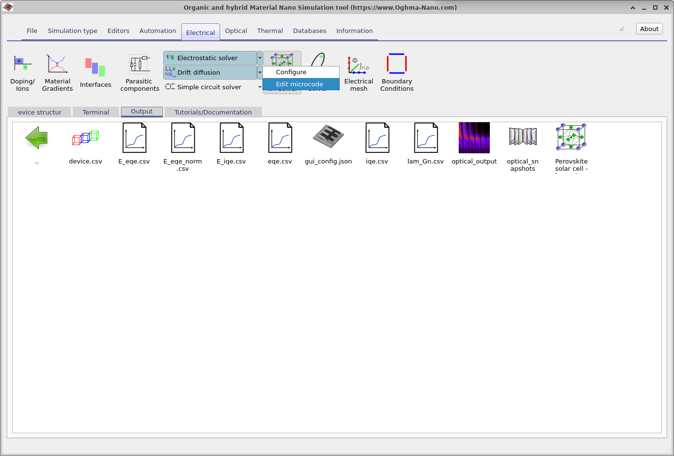
Practically, in OghmaNano there are two ways to deal with mobile ions when running EQE. The first is to disable the mobile-ion solver completely. This can be done from the Electrical ribbon in the main window by un-pressing the Perovskite ion solver button, which sits just under the menu shown in ??. The drawback of this approach is that it ignores ion motion entirely.
The second, and more subtle, method is to let the ions remain mobile during the slow voltage ramp, so they stabilise into a quasi-equilibrium distribution, and then “freeze” them only when the EQE measurement itself begins. This is equivalent to experimentally applying a slow negative voltage ramp to let the ions settle, and then measuring EQE very quickly before the ions have time to move. In the provided simulation this is done by default via a small Lua script.
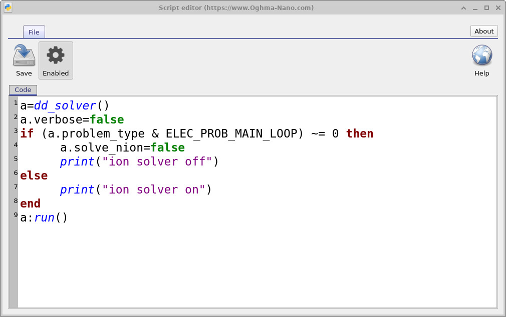
To view or edit this behaviour, go to the Electrical ribbon, open the menu to the right of the Drift diffusion button, and click Edit microcode (see ??). This opens the script editor window (??), which shows the Lua code controlling the solver. The key lines switch the ion solver off whenever the EQE calculation is running, but keep it on during the voltage ramp. This ensures that ions reach equilibrium before EQE is computed, giving consistent and physically realistic results. The same trick can also be applied to JV curves or other experiments.
📝 Task 1 — EQE as a function of bias
Goal: See how bias affects EQE and why more negative voltages suppress recombination artefacts.
- Open the EQE editor: Main window → Editors → EQE.
- Set EQE Voltage to
-1V and run the EQE simulation. - Sweep the following voltages, re-running EQE each time and saving the spectra:
+1 V → +0.5 V → 0 V → −1 V → +3 V → +5 V. (Forward bias, e.g. +3 V and +5 V, will intentionally increase recombination and depress EQE.) - Overlay the spectra and note where the curves diverge most (near the absorption edge, long-wavelength roll-off, etc.).
Expected observations / results
- At −1 V, EQE is typically highest and smoothest (collection aided; minimal recombination).
- At 0 V (JSC), EQE usually drops slightly vs −1 V, particularly near the band-edge.
- At +0.5 V and +1 V, increased recombination reduces EQE further.
- At stronger forward bias (+3 V, +5 V), EQE can fall sharply and may no longer represent intrinsic EQE (it becomes recombination-limited).
- The wavelength region most sensitive to bias is often the long-wavelength tail (where absorption is weaker and carrier collection matters most).
🧪 Task 2 — EQE at JSC with varying recombination
Goal: Quantify how recombination impacts the EQE spectrum under short-circuit conditions.
- Set EQE Voltage to
0V (i.e., JSC) in the EQE editor. - In the device’s Electrical parameters, locate trap-assisted (SRH) recombination settings (e.g., carrier lifetimes, capture cross-sections, or defect density).
- Run three simulations:
- Baseline: current/default recombination values.
- Higher recombination: increase SRH rate ~×10 (shorter lifetimes or larger cross-sections).
- Lower recombination: decrease SRH rate ~÷10 (longer lifetimes or smaller cross-sections).
- Compare the three EQE spectra (focus on the long-wavelength onset and any features near optical interference peaks).
Expected observations / results
- Higher SRH recombination → reduced EQE, most evident near the absorption edge and in regions with weak generation.
- Lower SRH recombination → EQE approaches the optical “ceiling” set by absorption/optics.
- Changes may mimic thickness/optical effects; use both
eqe.csv(λ-domain) ande_eqe.csv(E-domain) to diagnose.
ℹ️ Note: For clean EQE extraction, prefer mild reverse bias (e.g., −1 V) to minimise recombination. Forward-bias conditions (+3 to +5 V) are illustrative but typically not representative of intrinsic EQE.
✅ What you’ve learned
- How to set up and run an EQE simulation in OghmaNano.
- Where to find and plot the results (
eqe.csvande_eqe.csv). - Why perovskites need special treatment because of mobile ions.
- How to choose the EQE voltage, and why more negative voltages minimise recombination.
- Two approaches to handling mobile ions: disable them completely, or freeze them only during the EQE step.
👉 Next steps:
- Return to the perovskite solar cell simulation guide for the full tutorial overview.