Suns–Jsc Tutorial: Extracting photocurrent scaling from illumination intensity
Introduction
Suns–Jsc is the counterpart to Suns–Voc, but instead of tracking the open-circuit voltage, the experiment records the short-circuit current density Jsc as a function of illumination intensity (Suns). Because Jsc is directly proportional to photogeneration in the ideal case, this method is widely used to check for collection efficiency, identify current saturation, and reveal the impact of recombination or transport bottlenecks under strong illumination.
In an ideal device with efficient charge extraction, Jsc should increase linearly with Suns. Deviations from linearity—such as sub-linear growth at high intensities—indicate recombination losses, poor carrier mobility, or series-resistance limitations. Super-linear behaviour at very low intensities may indicate trap filling or photoconductive gain.
In practice, Suns–Jsc is performed by sweeping the light intensity across a chosen
range (e.g. 0.01–10 Suns) while holding the device at short circuit.
OghmaNano saves the results into suns_jsc.csv, which can be plotted to
reveal how well the device maintains collection efficiency across orders of magnitude
of illumination. By fitting the slope on a log–log scale, one can identify whether
the scaling is linear (α ≈ 1) or limited by recombination/transport effects.
Suns–Jsc analysis is therefore a useful complement to JV and Suns–Voc measurements: it isolates current-collection processes and highlights when carrier extraction or transport become limiting.
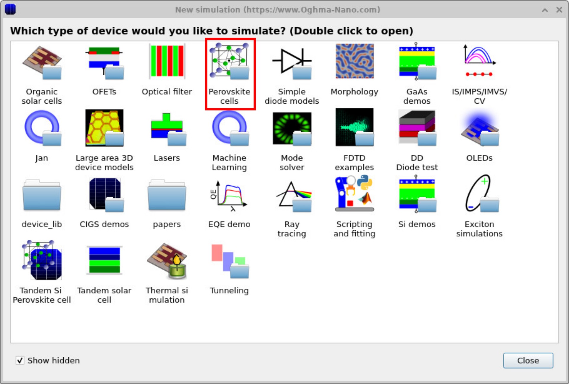
Step 1: Making a new simulation
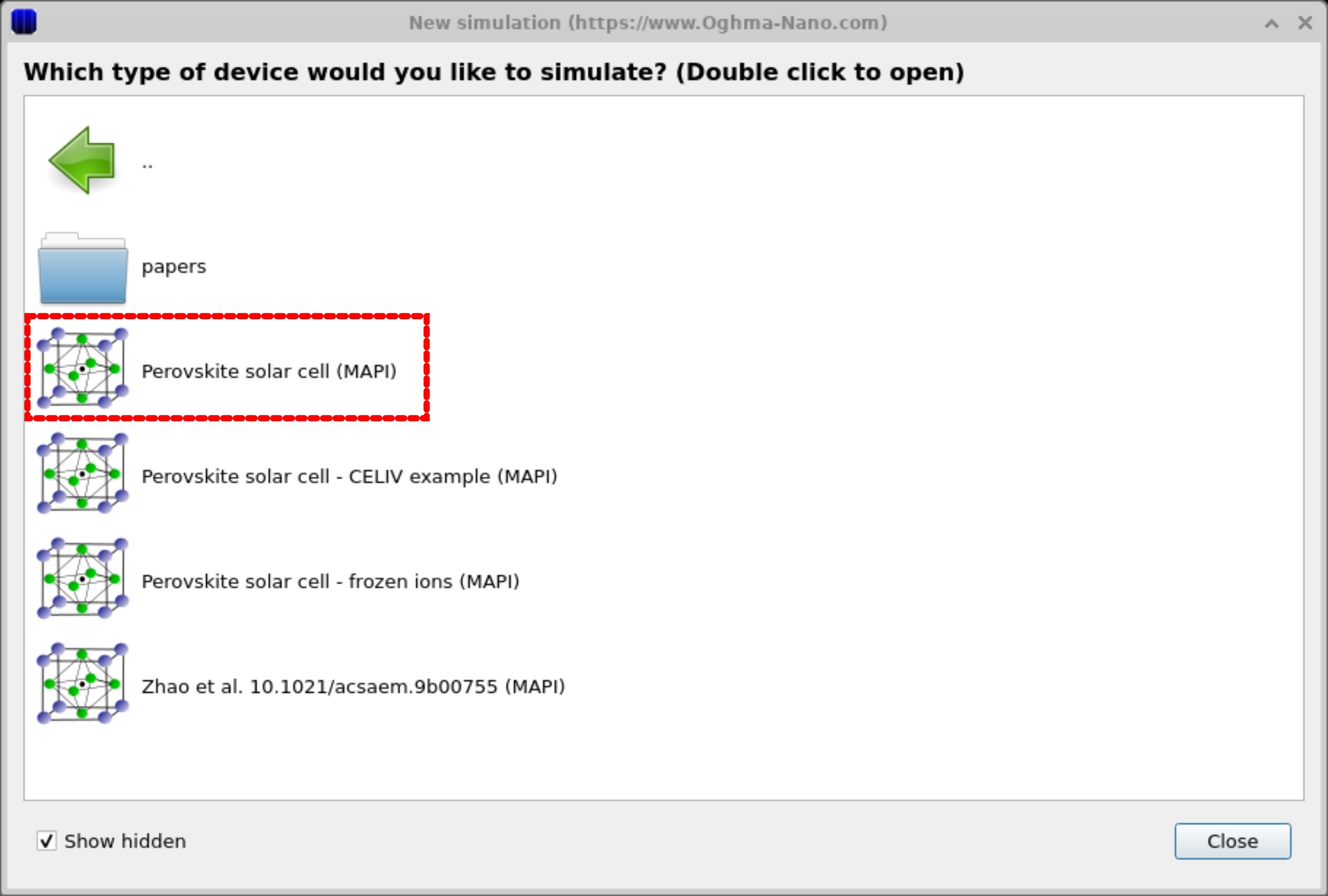
Double-click the Perovskite cells category in the new simulation window (??), then choose Perovskite solar cell (MAPI) (??) and save the project to disk. Although this tutorial uses the MAPI example, the Suns–Jsc procedure applies to any solar cell structure, since it simply varies the light intensity and measures the resulting Jsc.
Step 2: Selecting the simulation mode
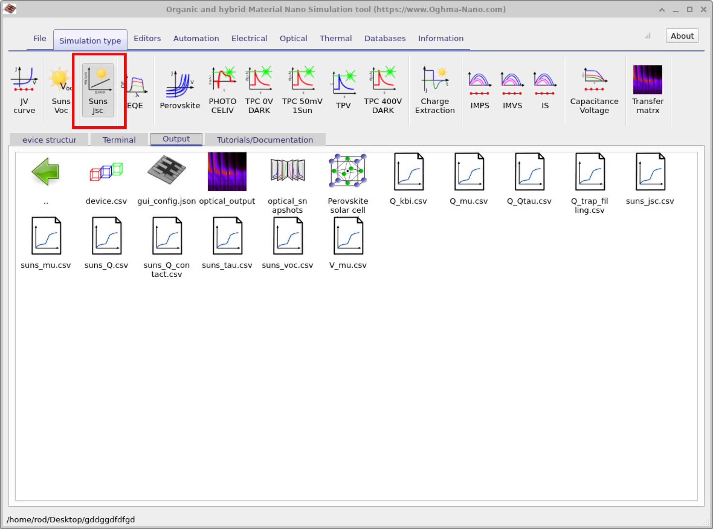
After saving, the main simulation window opens. Switch the simulator into Suns–Jsc mode by going to Simulation type and clicking the Suns–Jsc button so it appears pressed (??). Running the simulation in this mode generates a Suns–Jsc curve.
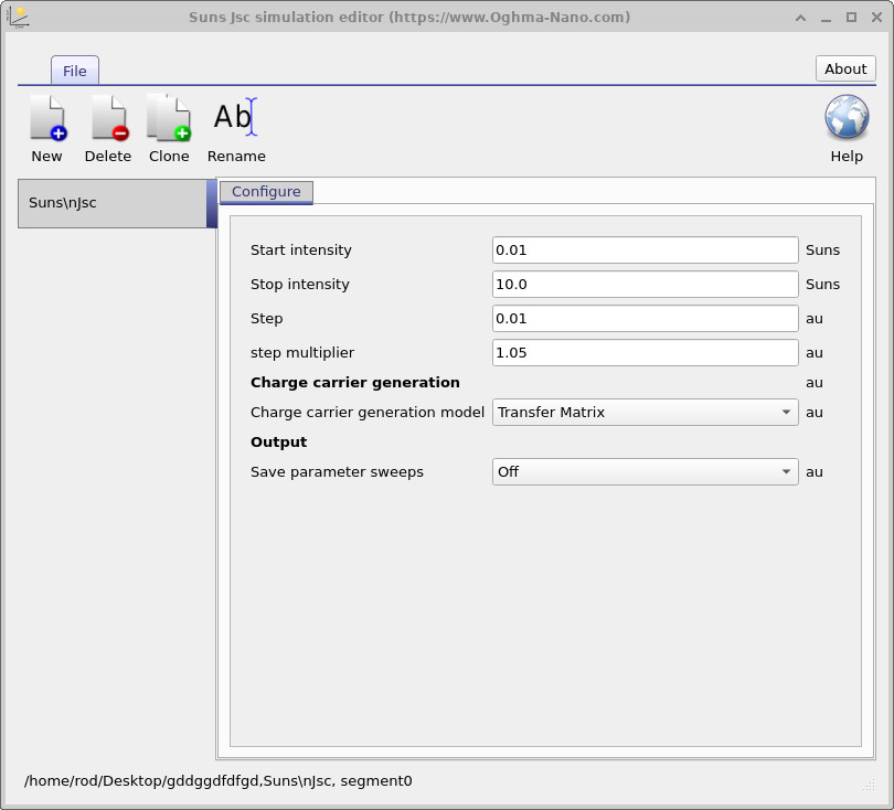
To configure the Suns–Jsc experiment, open the Editors ribbon and select Suns–Jsc (not shown here). This opens the configuration window (??), where you can set the start intensity, stop intensity (in Suns), and the step multiplier. The step multiplier (e.g. 1.2) scales intensity logarithmically, which makes it easier to inspect Jsc scaling on log–log plots. For example, the stop intensity here is 1.1 Suns, but in practice one might extend to ~10 Suns to test saturation. The defaults are usually fine for a first run.
Step 3: Looking at the results
Once configured, return to the main window and click Play (or press F9).
When the run finishes, open the Output tab
(??)
and locate suns_jsc.csv. Opening this file produces the Suns vs. Jsc plot
(??).
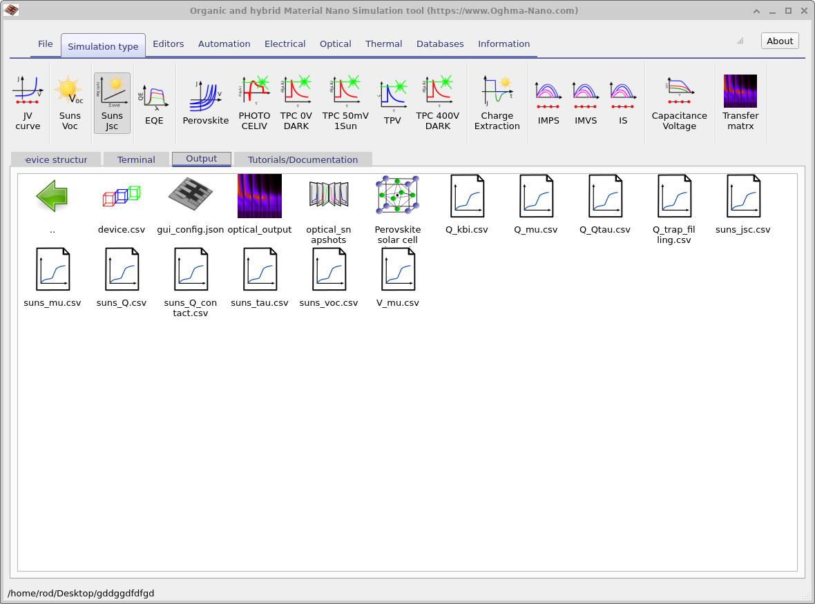
suns_jsc.csv.
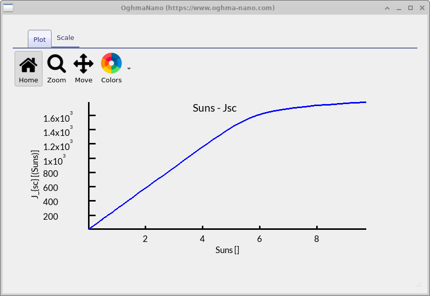
suns_jsc.csv displays the Suns vs. Jsc curve.
You have now run a Suns–Jsc simulation and produced the characteristic curve. This curve shows how the photocurrent scales with light intensity, providing a direct check of collection efficiency and possible saturation. To deepen your understanding, experiment with the electrical parameters: changes in traps, recombination rates, or mobilities will noticeably affect the scaling behaviour.
📈 Advanced: Analyse your Suns–Jsc curve — click to expand
Goal; quantify how Jsc scales with illumination. On a log–log plot, fit a straight line to obtain the exponent α in \( J_{sc} \propto \text{Suns}^{\,\alpha} \).
Interpretation; \(\alpha \approx 1\) → efficient collection (no saturation); \(\alpha < 1\) → recombination/transport limits at higher carrier density; \(\alpha > 1\) at very low Suns can indicate trap filling or photoconductive gain.
👉 Next steps:
- Now continue to SCLC mobility extraction.
- Return to the perovskite solar cell simulation guide for the full tutorial overview.