Quick start: Using Solar Spectra in J–V Simulations
In this quick start we take the solar spectra generated with OghmaNano’s Solar Spectrum Generator and use them as inputs for photovoltaic device simulations. By importing spectra into the simulator, we can run J–V curves and directly compare how devices behave under different illumination conditions (e.g. AM1.5G, polluted atmosphere, morning vs. noon sun).
1. Introduction:
In Part A, we saw how spectra vary with time of day, season, latitude, and air quality. In this section, we will import those spectra into the simulator to examine their impact on device performance. Because the normalisation bug has been fixed, each spectrum now retains its absolute irradiance. This means that both the shape of the spectrum (e.g. UV suppression by aerosols, IR absorption by water vapour) and the total intensity influence the J–V results.
This approach lets us answer practical questions, such as:
- How does heavy pollution (high aerosol optical depth) reduce photocurrent?
- What seasonal or diurnal effects are visible in the J–V curve?
- How sensitive is an organic solar cell to the spectral shape compared to its total irradiance?
By linking spectra directly into J–V simulations, we bridge the gap between solar irradiance modeling and device performance analysis, making it possible to test realistic operating conditions beyond the AM1.5G standard.
2. Getting started:
This tutorial continues directly from the previous section
(see Part A).
Please make sure you have completed that tutorial before starting here.
We will assume that you have already generated a new spectrum called Example
using the Solar Spectrum Generator. Open the example spectrum in the Optical Spectrum Editor.
In this part of the tutorial, our goal is to create a spectrum that looks
very different from the standard AM1.5G reference. To do this, you can
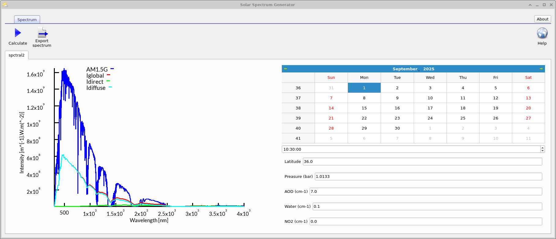
adjust any of the input parameters — such as time of day, date, latitude,
atmospheric water content, or aerosol optical depth. In the example below,
the aerosol optical depth (AOD) has been set to 7.0,
producing a much weaker Iglobal and Idiffuse
profile compared to AM1.5G
(see ??).
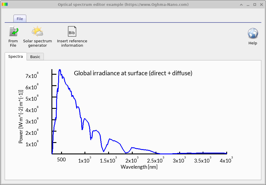
Once you have adjusted the parameters and generated your new spectrum,
click the Export spectrum button to save it into the model.
The spectrum will automatically be imported back into the Optical Spectrum Editor,
where it is added under the name Example.
This can be seen in
??.
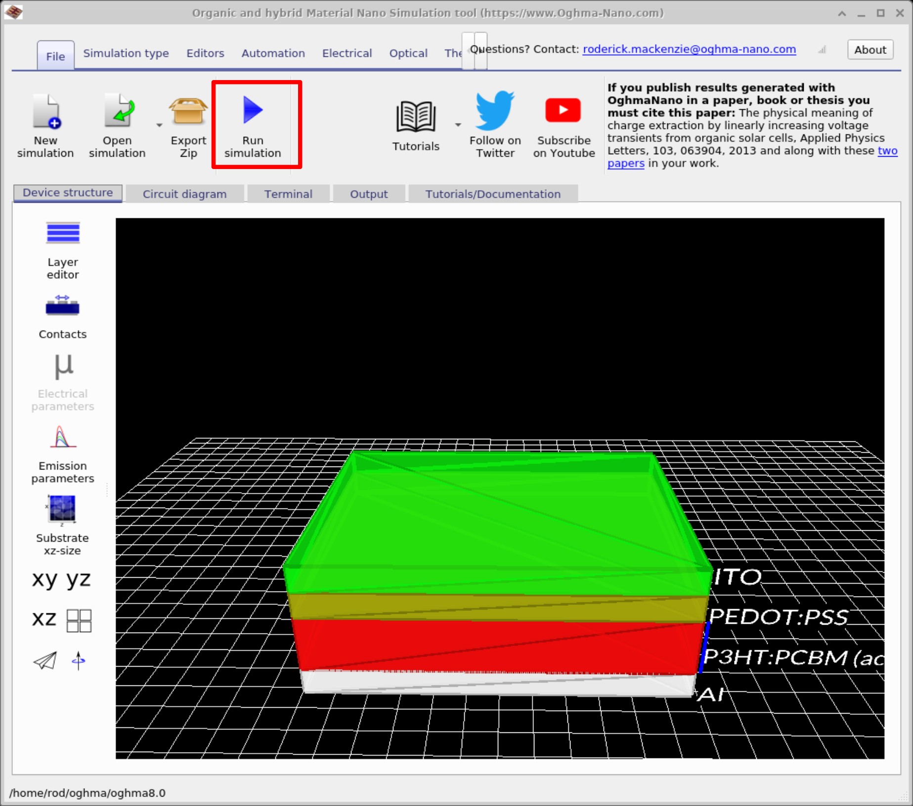
3. Running the baseline simulation
Before we use the custom solar spectrum you generated, let’s run a baseline electrical simulation to establish the device’s current performance. We’ll then compare the results to the run that uses your new spectrum.
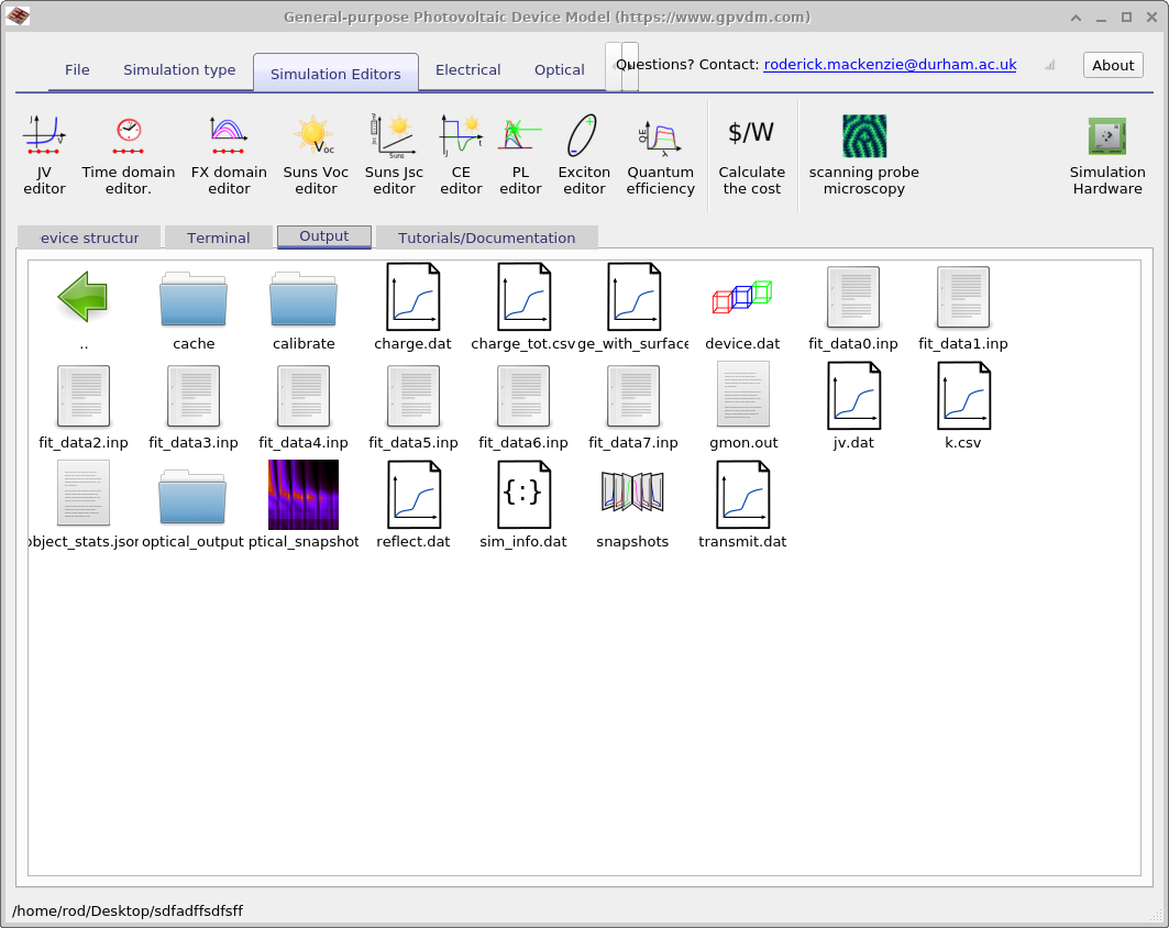
jv.csv or jv.csv, depending on your setup) and sim_info.dat.
Note the device’s VOC, JSC, and fill factor
to use as your baseline.
4. Using your generated spectra
Now we’ll use the spectrum you created (e.g., Example) in a device simulation.
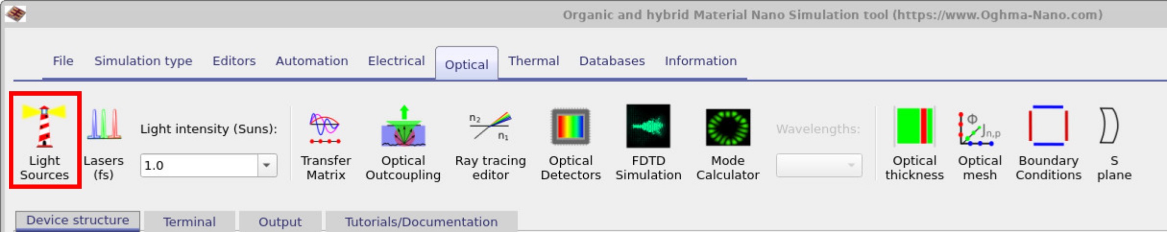
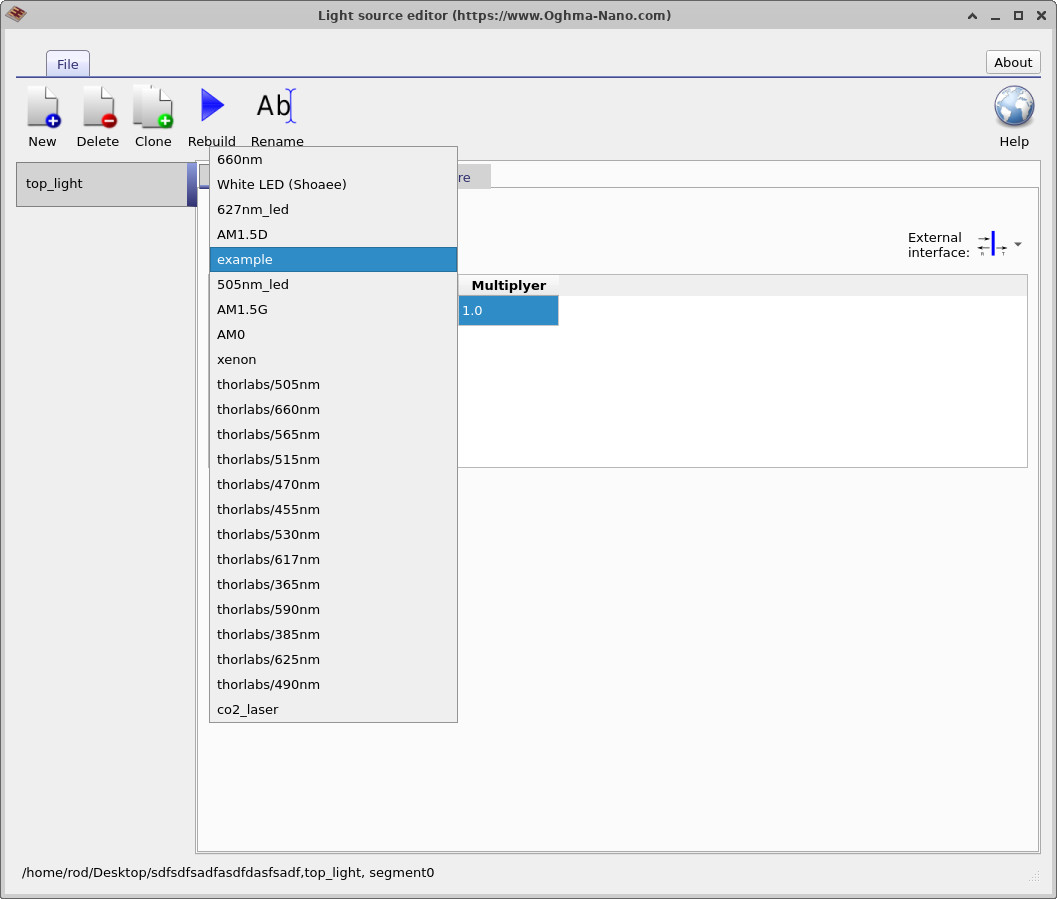
Open the Optical ribbon and click Light Sources to open the
Light Source editor. Change the spectrum from AM1.5G to example, then
re-run the electrical simulation. Finally, review jv.csv (or jv.csv)
and sim_info.dat to compare the updated PCE,
VOC, and JSC against your baseline.
jv.csv (or jv.csv) and sim_info.dat for changes in
PCE, VOC, and JSC.
📝 Try it yourself
Use your Example spectrum in the Solar Spectrum Generator and vary the parameters below.
After each change, click Calculate, then Export spectrum and re-run the J–V simulation.
Compare how PCE, VOC, and JSC change against your baseline.
- Increase aerosol optical depth (AOD) from 0.1 → 2.0 → 7.0.
- Change water vapour content from dry (0.1 cm) to humid (5 cm).
- Shift the time of day from noon to late afternoon.
- Change latitude (e.g. 0° equator, 50° London, 70° Arctic circle).
- Vary air pressure/altitude from sea level to 3000 m.
✅ Expected trends
- AOD: Higher aerosol levels scatter and absorb more light, reducing total irradiance. Idirect drops sharply; Idiffuse increases. Expect lower JSC and PCE overall.
- Water vapour: Adds absorption bands in the near-IR. These cut into spectral regions important for organic PV, leading to a modest drop in JSC and efficiency.
- Time of day: Morning/afternoon (higher air mass) red-shifts the spectrum and lowers total intensity. Voc may decrease slightly due to lower irradiance.
- Latitude: Higher latitudes increase air mass (on average), leading to lower irradiance and stronger seasonal variation. Equatorial spectra are more intense and balanced across wavelengths.
- Altitude: At higher elevations, there is less atmosphere above you. This increases direct irradiance and reduces scattering losses, so JSC increases compared to sea level.
These effects illustrate how environmental conditions directly affect photovoltaic device performance.
What you’ve learned in this tutorial
- How to generate custom solar spectra with the Solar Spectrum Generator in OghmaNano.
- The differences between AM1.5G, Iglobal, Idirect, and Idiffuse spectra.
- How environmental conditions (aerosols, water vapour, pollution, time of day, latitude) reshape the spectrum.
- How to export a spectrum into the Optical Spectrum Editor and use it as a light source in simulations.
- How to compare baseline vs. custom spectrum J–V results and evaluate changes in PCE, VOC, and JSC.
🎯 By completing Part B, you’ve connected solar irradiance modeling to device-level performance, moving from physical spectra to photovoltaic efficiency analysis.