Automation and Scripting
Often a user will have set up a simulation structure to represent a real world device but will then ask the question: What happens to my solar cell efficiency as I change the mobility of the active layer? Or what happens to the wavelength of my laser output as I change the thickness of the Quantum Well. To answer these type of questions one must change one or more material parameters over a range of values and then examine the simulation results. Clearly this could be done by hand but there are better ways to automate this process.
There are three main ways to automate OghamNano simulations:
-
The first method is using the parameter scan window, this is described below in section 17.1. The parameter scan window allows a user to vary a parameter (or multiple paramters) in steps using the graphical user interface. No knowledge of coding is required for this approach. The parameter scan window is useful if one wants to quickly examine how a parameter influences the results and the scenario you are examining is not very complex. The scan window fits most users’s needs most of the time.
-
For more fine grained control over how the parameters are varied the next method is to use Python scripting, this is described in section 17.4. Python scripting allws the user ultimate flexibility in adjusting all simulation parameters and running simulations, Python is widely available which makes this approach very attractive.
-
The third way is through MATLAB scripting, this is described in section 17.4.3. The advantage of MATLAB scripting is that lots of people can code in MATLAB so makes automating OghmaNano very accessable. The downside of using MATLAB is that it is quite expensive and not all people have access to it. An alternative to MATLAB would be Octave however at the time of writing it does not have a json reader/writer.
Or option 4: All the above methods rely on the same principles: The OghmaNano simulation save file is systematic edited and the back end of the software \(oghma\_core.exe\) run on the sim.oghma file to generate new results. Key to understanding how scripting works is to realize that the sim.oghma is simply a zip file (See 14.1) with a json file (sim.json) inside it, and if one can edit the json file (using any language you want ActionScript, C, C++, C#, Cold Fusion, Java, Lisp, Perl, Objective-C, OCAML, PHP, Python, Ruby etc... ) the you can automate OghmaNano.
The parameter scan window
Related YouTube videos:
 |
Using the parameter scan tool in OghmaNano |
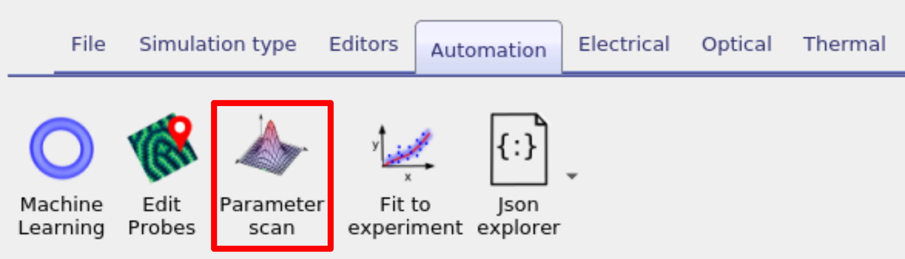
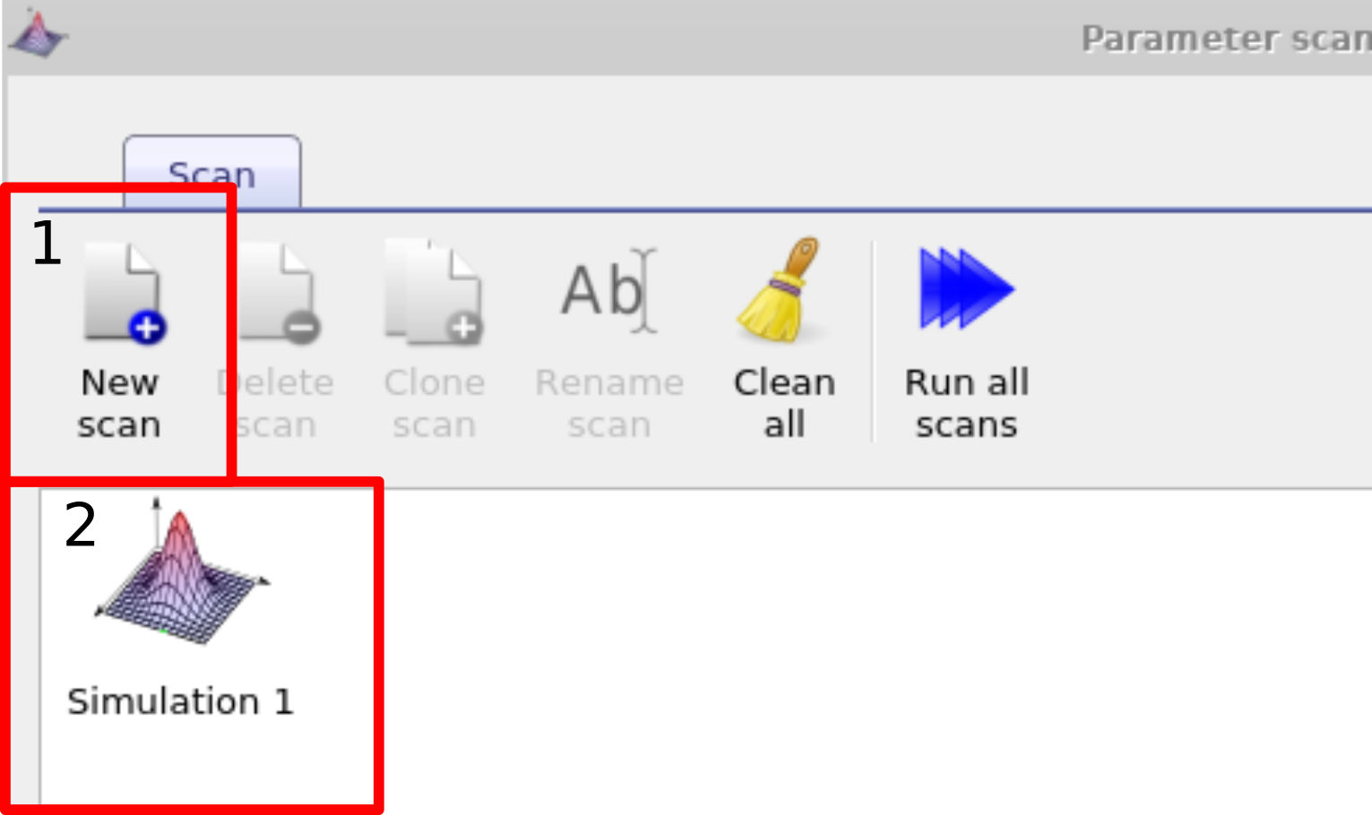
The most straight forward way to systematically vary a simulation parameter is to use the scan window. In this example we are going to systematic change the mobility of the active layer of a PM6:Y6 solar cell, you can find this example in the example simulations under Scripting and fitting/Scan demo (PMY:Y6 OPV). Once you have located this simulation and opened it, you then need to bring up the parameter scan window, this can be done by clicking on the Parameter scan icon in the Automation ribbon (see Figure [fig:parameter_scan_icon]). Then make a new scan by clicking on the new scan button (1) (In the example simulation this has already been done for you). Open the new scan by double clicking on the icon representing the scan (2), see figure [fig:newscan]. This will bring up the scan window, see figure 17.1.
 [fig:parameter_scan_icon]
 [fig:newscan]
Changing one material parameter
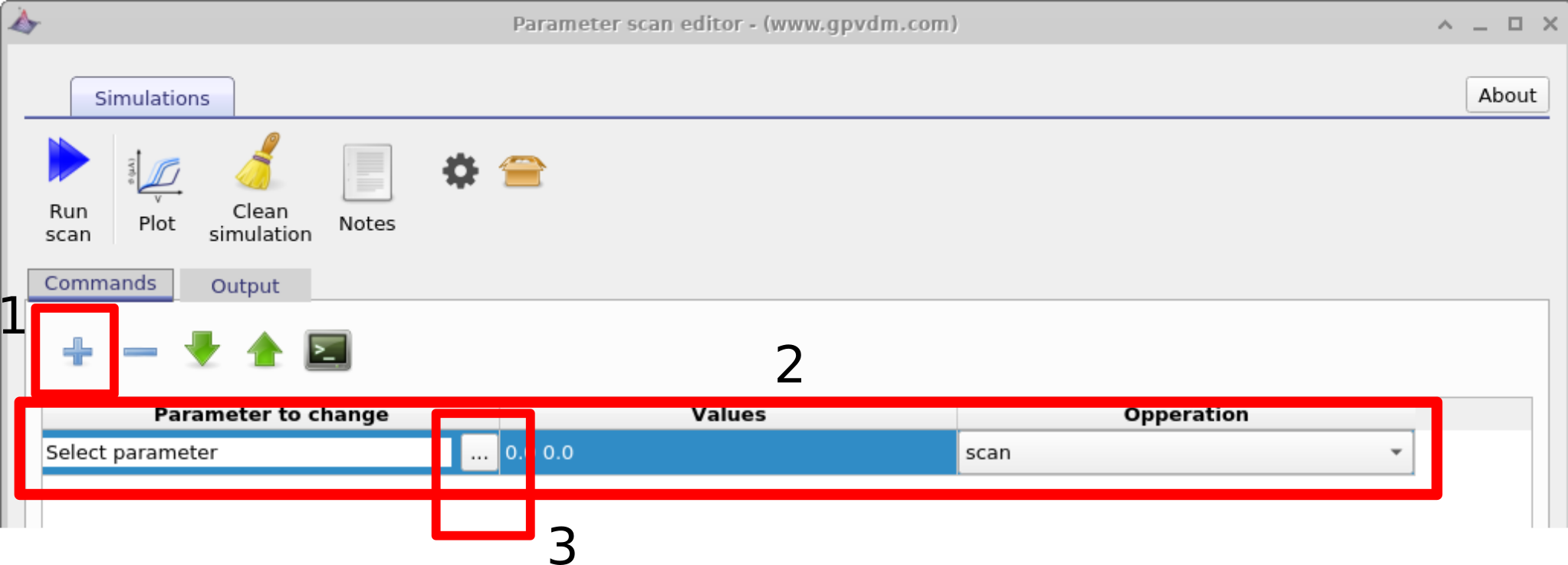
Once the scan window has opened, make a new scan line by clicking on the the plus icon (1) in figure 17.1, then select this line so that it is highlighted (2), then click on the three dots (3) to select which parameter you want to scan. Again if you are using the example simulation this will already have been done for you.
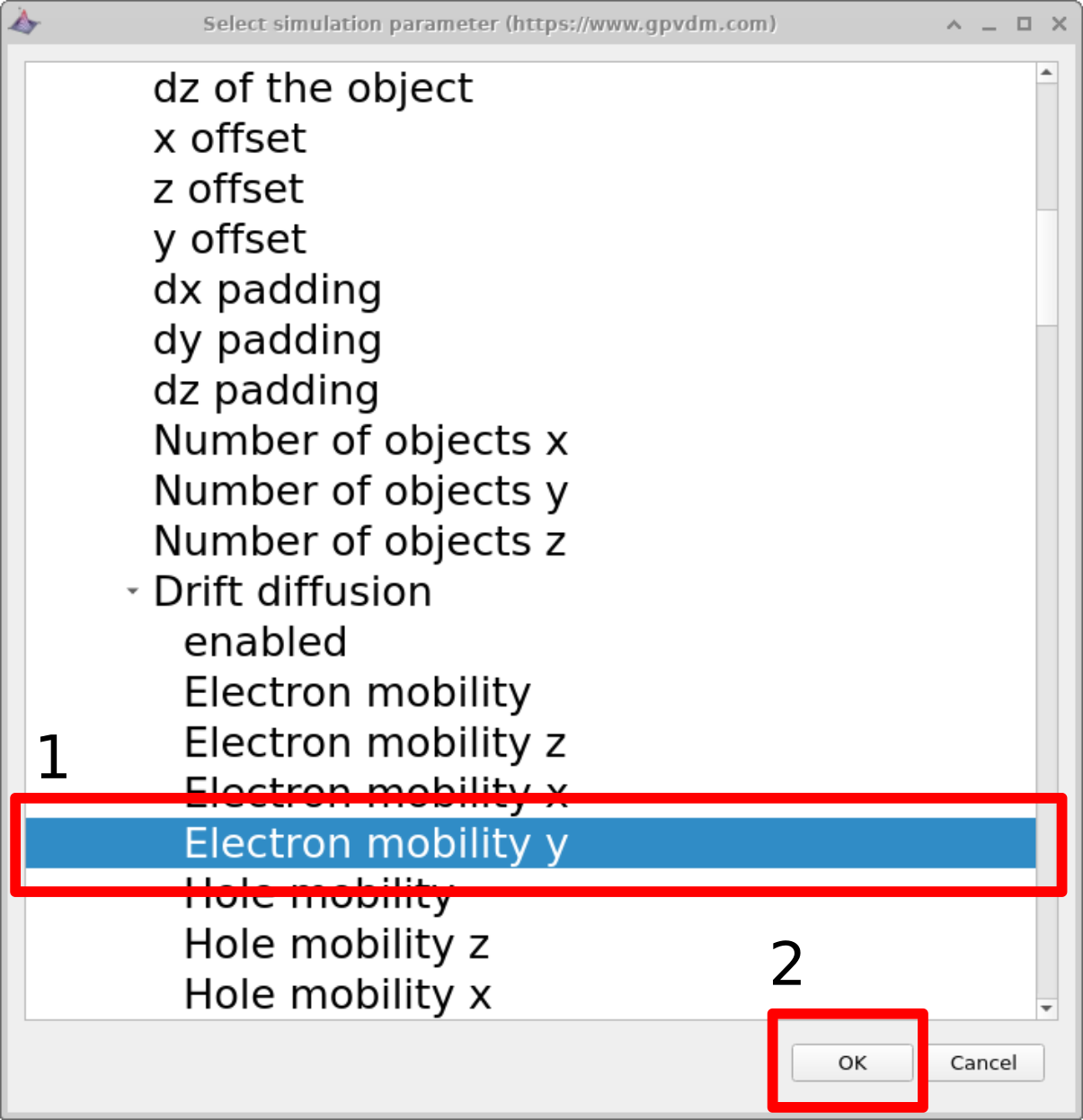
In this example we will be selecting the electron mobility of a PM6:Y6 solar cell. Do this by navigating to epitaxy\(\rightarrow\) PM6:Y6\(\rightarrow\) Drift diffusion\(\rightarrow\) Electron mobility y. Highlight the parameter and then click OK. This should then appear in the scan line. The meaning of epitaxy\(\rightarrow\) PM6:Y6\(\rightarrow\) Drift diffusion\(\rightarrow\)Electron mobility y will now be explained below:
-
epitaxy: All parameters in the .oghma file are exposed via the parameter selection window see [fig:scanselect]. This file is a tree structure, see 14.1. The device structure is defined under the heading epitaxy.
-
PM6:Y6: Under epitaxy each layer of the device is given by its name. The active layer in this device is called PM6:Y6, if your active layer was called Perovskite or P3HT:PCBM you would have selected this instead.
-
Drift diffusion: All electrical parameters are stored under the sub heading drift diffusion.
 [fig:scanselect]
-
Electron mobility y: One can define asymmetric mobilities in the z,x and y direction - this is useful for OFET simulations. However by default the model assumes a symmetric mobility which is the same in all directions. This value is defined by Electron mobility y.
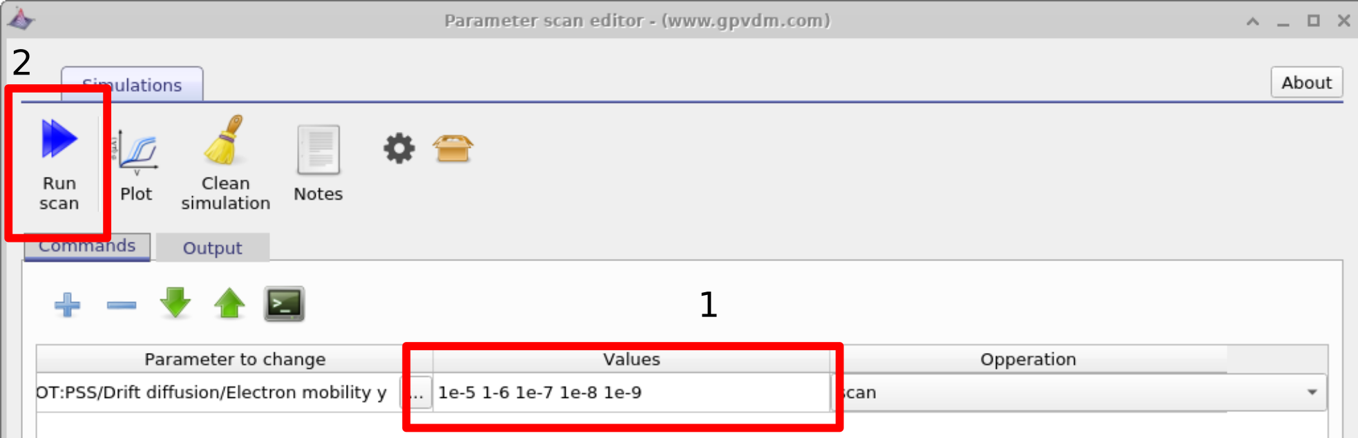
Next enter the values of mobility which you want to scan over in this case we will be entering 1e-5 1-6 1e-7 1e-8 1e-9 (see figure 17.2 1) then click run scan (see figure 17.2 2). OghmaNano will run one simulation on each core of your computer until all the simulations are finished.
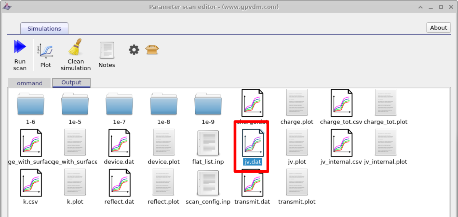
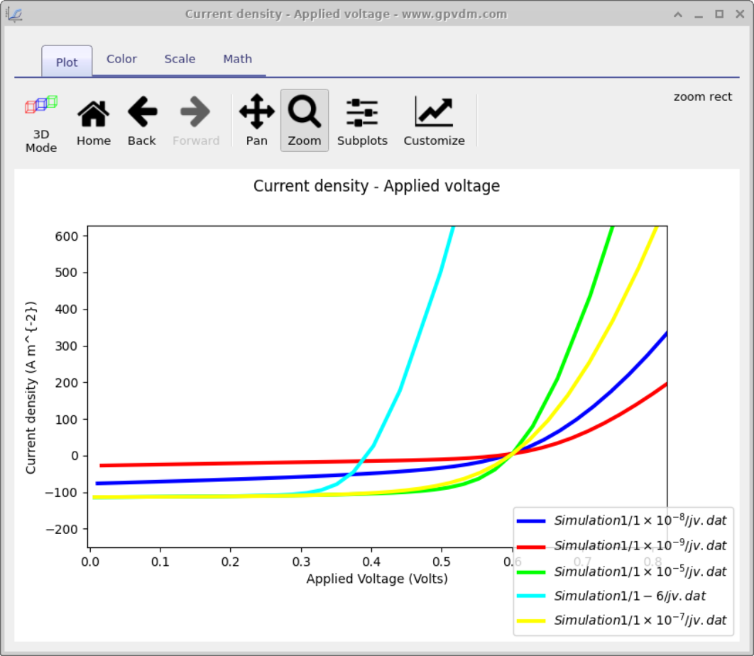
To view the simulation results click on the output tab this will bring up the simulation outputs, see figure 17.3. You can see that a directory has been created for each variable that we scanned over so 1e-5, 1e-6, 1e-7, 1e-8 and 1e-9. If you look inside each directory it will be an exact copy of the base simulation directory. If you double click on the files with multi-colored JV curves, see the red box in figure 17.3. OghmaNano will automaticity plot all the curves from each simulation in one graph, see figure 17.4.
Duplicating parameters - changing the thickness of the active layer
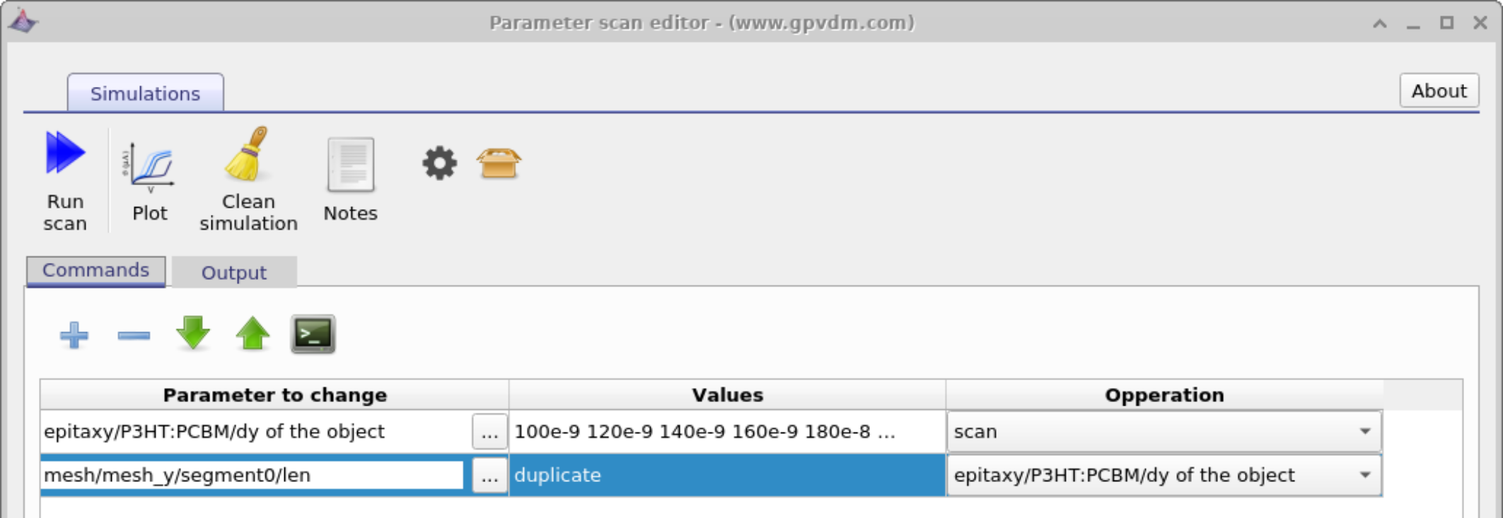
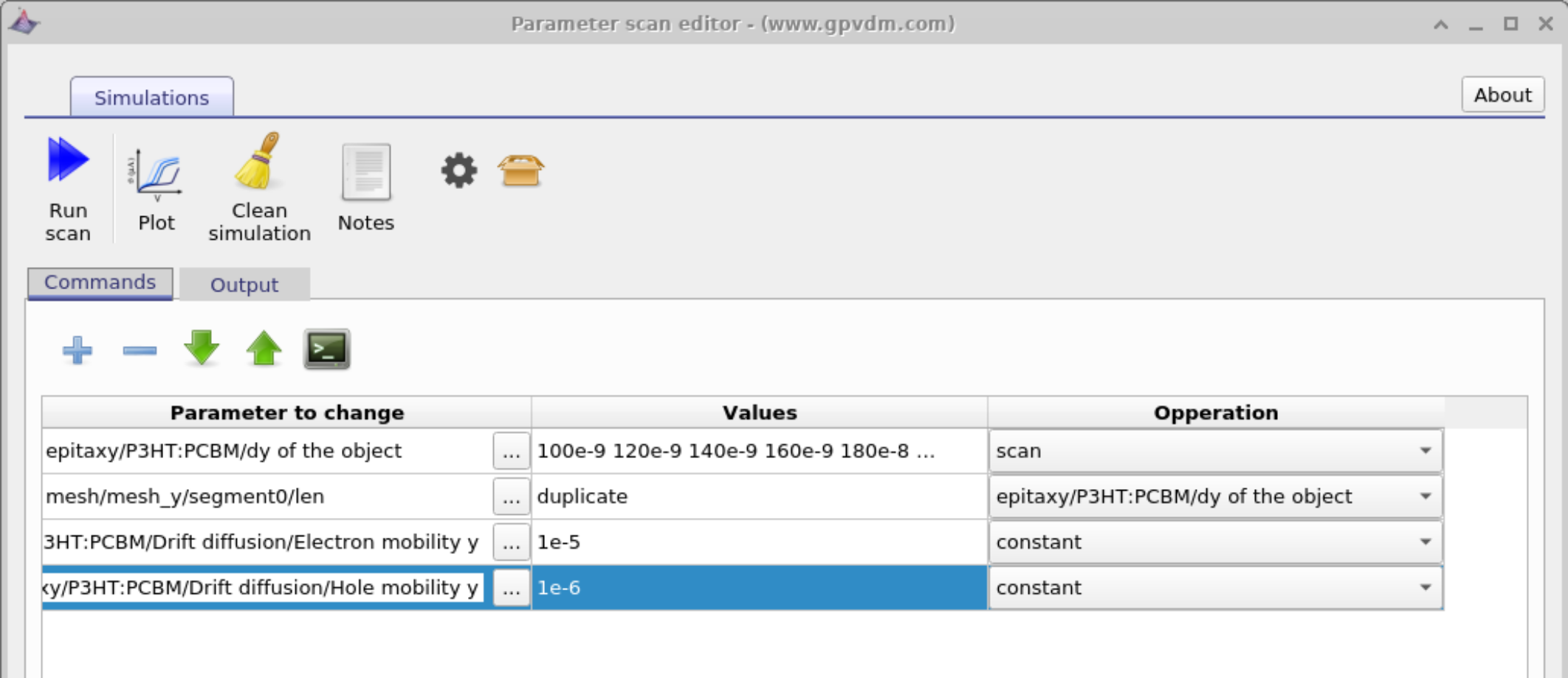
Very often one wants to change a parameter, then set another parameter equal to the parameter which was changed. An example of this is one may want to change electron and hole mobilities together when simulating a device with symmetric mobilities. This can be done using the duplicate function of the scan window as seen in figure 17.5. In this example we tackle a slightly more tricky problem than changing mobilities together we are going to change the physical width of the active layer and at the same time adjust the electrical mesh to make it match. As discussed in section 8 the width of the active layer must always match the width of the electrical mesh. When you change the layer width by hand in the layer editor OghmaNano updates the width of the electrical mesh for you. But when scripting the model it won’t do this update for you. Therefore in the example below we are going to set the width of the active layer by scanning over:
epitaxy\(\rightarrow\)PM6:Y6\(\rightarrow\)dy
of the object
Then we are going to add another line under and under parameter to scan select
mesh\(\rightarrow\)mesh_y\(\rightarrow\)segment0\(\rightarrow\)len
and set it to
epitaxy\(\rightarrow\)PM6:Y6\(\rightarrow\)dy of
the object
under the operation dropdown box. You will see the word duplicate appear under values.
If you now run the simulation "epitaxy\(\rightarrow\)PM6:Y6\(\rightarrow\)dy of the object" will be changed and "mesh\(\rightarrow\)mesh_y\(\rightarrow\)segment0\(\rightarrow\)len" will follow it.
Side note: Device with multiple active layers
The sum of the active layer thickness (as defined in the layer editor) MUST equal the electrical mesh thickness (more about the mesh in section 8). If for example one had three active layers TiO2 (100 nm)/Perovskite (200 nm)/Spiro (100 nm) with a total width of 400 nm. The total mesh length must be 400 nm as well. Therefore were one want to change the thickness of the perovskite layer as in 17.5 one would have to break the electrical mesh up into three sections and make sure you were updating the mesh segment referring to the perovskite layer alone.
Setting constants
Often when running a parameter scan one wants to set a constant value, this can be done using the "constant" option in the Operations dropdown menu. See figure 17.6
The equivalent of loops
Often when scanning over a parameter range one may want to simulate so many parameters that it is not practical to type them in. In this case OghmaNano has the equivalent of a loop. So for example if one wanted to change a value from 100 to 400 in steps of 1, one could type
[100 400 1]Limitations of the scan window
Although the scan window is convenient in that it provides a quick way to scan simulation parameters, it is by nature rather limited in terms of flexibility. If you want to do complex scans were multiple parameters are changed or to programmatically collect data from each simulation then you can use the or matlab interfaces to OghmaNano. These are described in the latter sections.
Multiparameter device optimizer
Related YouTube videos:
|
Optimizing the layer structure of a Perovskite solar cell |
|
Optimizing an OPV device for maximum photon harvesting. |
|
Searching for the optimum layer structure in an organic solar cell. |
Very often when optimizing a device an engineer or scientists will be want to know what the optimum structure of a device is. For example a perovskite solar cell is made up of multiple layers, but what is the optimum thickness of each layer? If the perovskite layer is made really thick then lots of light will be absorbed but the down side of this is that it will take longer for charge carriers to escape the device so recombination will be high. Conversely if the layer is made really thin very few carriers will have a chance to recombine as they will not spend long in the device but the downside is that not many photons will be absorbed in the first place as the layer is thin. If one then also considers that light will reflect multiple times of interfaces in the device setting up standing wave pattens, this will further complicate the optimization problem as one will need to optimize not only the thickness of the perovskite layer but also the thicknesses of all other layers at the same time. To solve this multi-parameter optimization problem one can use the Fast optimizer within the scan window.
Using the multi parameter optimizer
In the new simulation window under the sub-topic Scripting and fitting there are several examples of multi-parameter optimizers:
-
Electrical layer optimizer: This will vary the layer thickness of two active layers of an organic solar cell simulation and plot the PEC/FF/Voc as a function of these layer thicknesses.
-
Optical layer optimizer (perovskite): This will vary the thickness of two layers in a perovskite solar cell and plot the current generated by each layer within the device.
-
Optical layer optimizer (OPV): This will vary the thickness of two layers in a perovskite solar cell and plot the current generated by each layer within the device.
In this text we will be using the Optical layer optimizer (perovskite), if you open this simulation and navigate to the scan window, you will see a scan already set up called optimizer. If you open it you will get a window shown in figure 17.7. This scan window looks just like the scan windows described in the previous section, however the key difference is that the Fast optimizer button is depressed. When this button is depressed scan results are not written to disk, instead the key simulation parameters are tabulated and saved to disk at the end of the simulation. Notice that in this example we are varying the thickness (dy) of the Perovskite layer between 300nm and 500 nm in steps of 10 nm and the thickness (dy) TiO2 layer from 100 nm to 300 nm also in steps of 10 nm. Try running the simulation, the using windows explorer navigate to your simulation directory, then open the folder called optimize and in there you will find a csv file called optimizer_output.csv. If you open this with Excel or LibreOffice, it will look like figure 17.8.

If you examine figure 17.8 carefully you can see the first two columns are labelled epitaxy.layer2.dy and epitaxy.layer1.dy . These are the layer thicknesses we decided to change in the scan window. For every subsequent layer in the device there are two columns, labelled layerX/light_frac_photon_generation and layerX/J. These refer to the fraction of the light absorbed with in the layer and the maximum current this layer would produce if all the light absorbed within the layer were turned into current. Clearly if light is absorbed within the active layer it has a good chance of being turned into current, however if light is absorbed within the back metallic contact then there is little chance of that light being turned into electrical current. If you use the sorting tools included within Excel/LibreOffice you can figure out which device structures produce the most current.

opened in LibreOffice (You can use Excel). [fig:device_optimizer_output]
Python/MATLAB scripting of OghmaNano
Scripting offers a more powerful way to interact with gvpdm. Rather than using the graphical user interface, you can use your favourite programming language to interact with OghmaNano. This gives you the option to drive simulations in a far more powerful way than can be done using the graphical interface alone. Below I give examples of using MATLAB and python to drive OghmaNano, but you can use any language you want which has a json reader/writer. Pearl and Java are two languages which spring to mind.
Before you begin scripting OghmaNano you need to tell windows where OghmaNano is installed, the default OghmaNano will be installed to C:\Program files x86 \OghmaNano, in there you will see in this directory there are two windows executables, one called oghma.exe, this is the graphical user interface, and a second .exe, called oghma_core.exe. You can run oghma_core.exe from the command line without oghma.exe. You simply need to navigate to a directory containing a sim.oghma folder and call oghma_core.exe, this can be done from the windows command line, matlab, python or any other scripting language. However, before you can do this on windows, you need to add C:\Program files x86 \OghmaNano to your windows path so that windows knows where OghmaNano is installed. An example of how to do this on a modern version of windows is given in the link https://docs.microsoft.com/en-us/previous-versions/office/developer/sharepoint-2010/ee537574(v=office.14)
Every new version of windows seems to move the configuration options around, so you may have to find instructions for your version of windows.
Python scripting
Related YouTube videos:
|
Python scripting perovskite solar cell simulation |
There are two ways to interact with .oghmafiles via python, using native python commands or by using the OghmaNano class structures, examples of both are given below.
The native python way
As described in section 14.1, .oghmafiles are simply json files zipped up in an archive. If you extract the sim.json file form the sim.oghmafile you can use Python’s json reading/writing code to edit the .json config file directly, this is a quick and dirty approach which will work. You can then use the \(os.system\) call to run oghma_core to execute OghmaNano.
For example were one to want to change the mobility of the 1st device layer to 1.0 and then run a simulation you would use the code listed in listing [python-example].
       import json
       import os
       import sys

       f=open('sim.json')              #open the sim.json file
       lines=f.readlines()
       f.close()
       lines="".join(lines)    #convert the text to a python json object
     data = json.loads(lines)

     #Edit a value (use firefox as a json viewer
     # to help you figure out which value to edit)
     # this time we are editing the mobility of layer 1
     data['epitaxy']['layer1']['shape_dos']['mue_y']=1.0


     #convert the json object back to a string
     jstr = json.dumps(data, sort_keys=False, indent='\t')

     #write it back to disk
     f=open('sim.json',"w")
     f.write(jstr)
     f.close()

     #run the simulation using oghma_core
     os.system("oghma_core.exe")
If the simulation in sim.json is setup to run a JV curve, then a file called sim_data.dat will be written to the simulation directory containing paramters such as PCE, fill factor, \(J_{sc}\) and \(V_{oc}\). This again is a raw json file, to read this file in using python and write out the value of \(V_oc\) to a second file use the code given in listing [python-example2].
f=open('sim_info.dat')
lines=f.readlines()
f.close()
lines="".join(lines)
data = json.loads(lines)

f=open('out.dat',"a")
f.write(str(data["Voc"])+"\n");
f.close()
PyOghma
One can get a long way by manipulating the OghmaNano json files directly with python as described in 17.4.1. However, using this approach it is not possible (very easy) to run multiple simulations at the same time. And as most modern CPUs have 8 or more cores it seems a waste not to be running multiple simulations when generating large data sets. Furthermore, manipulating json files in Python is not very intuitive and not very python like. For this reason Cai Williams has written an API called PyOghma which can be used to manipulate OghmaNano json files and also run simulations. This is a stand alone project to OhgmaNano, so direct any questions about this to him!
PyOghma is available on GitHub and also via pip:
python -m pip install PyOghmaAn example of using PyOghma is given below [python-example3]:
 import PyOghma as po

       Oghma = po.OghmaNano()
       Results = po.Results()


       source_simulation = "\exapmle\pm6y6\"

      Oghma.set_source_simulation(source_simulation)

    experiment_name = 'NewExperiment'

    Oghma.set_experiment_name(experiment_name)

    mobility = 1e-5
    trap_desnsity = 1e-18
    trapping_crosssection = 1e-20
    recombination_crosssection = 1e-20
    urbach_energy = 40e-3
    temperature = 300
    intensity = 0.5


    experiment_name = 'NewExperiment' + str(1)
    Oghma.clone('NewExperiment0')

    Oghma.Optical.Light.set_light_Intensity(intensity)
    Oghma.Optical.Light.update()

    Oghma.Thermal.set_temperature(temperature)
    Oghma.Thermal.update()

    Oghma.Epitaxy.load_existing()
    Oghma.Epitaxy.pm6y6.dos.mobility('both', mobility)
    Oghma.Epitaxy.pm6y6.dos.trap_density('both', trap_desnsity)
    Oghma.Epitaxy.pm6y6.dos.trapping_rate('both', 'free to trap',..
    trapping_crosssection)
    Oghma.Epitaxy.pm6y6.dos.trapping_rate('both', 'trap to free',..
    recombination_crosssection)
    Oghma.Epitaxy.pm6y6.dos.urbach_energy('both', urbach_energy)
    Oghma.Epitaxy.update()

    Oghma.add_job(experiment_name)
    Oghma.run_jobs()
In this example PyOghma is imported as po, and a source OghmaNano json file is manipulated by changing the values of mobility, trap density, trapping rate and Urbach Energy. The original file is cloned with the line:
Oghma.clone('NewExperiment0')Then at the end of the code the following two lines. The first of which adds the job to the job list in PyOghma. And the second line tells PyOghma to execute all the jobs. If there were more than one job PyOghma would execute multiple jobs across all CPUs, until they were all finished. If for example one wanted to run simulations with different values of mobility, one would add each simulation to the jobs list, then call \(run\_jobs\) once to run the jobs across all cores in an efficient way.
Oghma.add_job(experiment_name)
Oghma.run_jobs()
More information about PyOghma is available on the GitHub page.
MATLAB scripting
As described in section 14.1 OghmaNano simulations are stored in .json files zipped up inside a zip archive. Matlab has both a zip decompressor and a json decoder. Therefore it is straight forward to edit and read and edit .oghma files in MATLAB. You can then use MATLAB to perform quite complex parameter scans. The example script below in listing [matlab-example] demonstrates how to run multiple simulations with mobilities ranging from 1e-7 to 1e-5 \(m^{2}V^{-1}s^{-1})\). The script starts off by unzipping the sim.json file, if you already have extracted your sim.json file from the sim.oghma file you don’t need these lines. The code then reads in sim.json using the MATLAB json decoder \(jsondecode\). A new directory is made which corresponds to the mobility value, the sim.oghma file copied into that directory. Then \(json\_data.epitaxy.layer0.shape\_dos.mue_y\) is set to the desired value of mobility and the simulation saved using \(jsonencode\) and \(fopen,fprintf,fclose\). The \(system\) call is then used to run \(oghma\_core.exe\) to perform the simulation. Out put parameters such as \(J_{sc}\) are stored in sim_data.dat again in json format, see section 4.1.4, although this is not done in this simple script.
if exist("sim.oghma", 'file')==false
 sprintf("No sim.oghma file found"); %Check if we have a sim.oghma file
end

if exist("sim.json", 'file')==false
 unzip("sim.oghma")  %if we don't have a sim.json file
                                      %try to extract it
end

A = fileread("sim.json");  %Read the json file.
json_data=jsondecode(A);  %Decode the json file

mobility=1e-7  %Start mobility
origonal_path=pwd  %working with the current dir
base_dir="mobility_scan"  %output directory name
while(mobility<1e-5)
    dir_name=sprintf("%e",mobility);
    full_path=fullfile(origonal_path,base_dir,dir_name)    %join paths
    mkdir(full_path)  %make the dir
    cd(full_path)  %cd to the dir

   %Update the json mobility
    json_data.epitaxy.layer0.shape_dos.mue_y=mobility  %Change mobility
                                                                                                      %of layer0

    copyfile(fullfile(origonal_path,"sim.oghma"),\\
           fullfile(origonal_path,base_dir,dir_name,"sim.oghma"))

   %now write the json file back to disk
    out=jsonencode(json_data);
    json_data
    fid = fopen("sim.json",'w');
    fprintf(fid, '%s', out);
    fclose(fid);

   %run oghma - This won't work if you have not added the oghma
   %install directory to your windows paths
    system("oghma_core.exe")

   %Multiply mobility by 10
    mobility=mobility*10;
end

%Move back to the original dir
cd(origonal_path)
The built in calculator
OghmaNano has a built-in calculator that can be used to perform simple mathematical operations. This functionality is useful for setting up fitting procedures and defining equations in various parts of the code. The calculator is based on Reverse Polish Notation (RPN).
Supported Operations
| Operation | Operator | Example |
|---|---|---|
| Exponentiation | ^ | 2 ^3 = 8 |
| Multiplication | \(*\) | \(2 * 3 = 6\) |
| Division | \(/\) | \(6 / 2 = 3\) |
| Addition | \(+\) | \(2 + 3 = 5\) |
| Subtraction | \(-\) | \(5 - 3 = 2\) |
| Greater than | \(>\) | \(5 > 3\) is 1 |
| Less than | \(<\) | \(2 < 5\) is 1 |
| Greater than or equal | \(>=\) | \(5 >= 5\) is 1 |
| Less than or equal | \(<=\) | \(3 <= 4\) is 1 |
Supported Functions
| Function Name | Function | Example |
|---|---|---|
| Sine | sin | \(\sin(\pi/2) = 1\) |
| Cosine | cos | \(\cos(0) = 1\) |
| Absolute Value | abs | \(\text{abs}(-3) = 3\) |
| Positive Value | pos | \(\text{pos}(-3) = 0, \text{pos}(3) = 3\) |
| Logarithm (base 10) | log | \(\log(100) = 2\) |
| Exponential | exp | \(\exp(2) = e^2\) |
| Square Root | sqrt | \(sqrt(9) = 3\) |
| Minimum | min | \(\min(2, 3) = 2\) |
| Maximum | max | \(\max(2, 3) = 3\) |
| Random | rand | \(\text{rand}(a, b)\) generates a random number between \(a\) and \(b\) |
| Log-random | randlog | \(\text{randlog}(a, b)\) generates a log-random number between \(a\) and \(b\) |