Suns–Voc Tutorial: Extracting recombination and ideality from Voc measurements

Introduction

Suns–Voc (also written as Sun–Voc) is a widely used characterisation method for solar cells, particularly for perovskites, organics, and other emerging thin-film technologies. The technique measures the open-circuit voltage (Voc) of a device as a function of illumination intensity (Suns). By gradually varying the incident light level, and recording the resulting Voc, we obtain a curve Voc(Suns) that reveals fundamental information about recombination and device physics.

At the most basic level, Voc scales with the logarithm of light intensity. According to the diode equation, \[ V_\text{oc} = \frac{n k_\text{B} T}{q} \ln\!\left(\frac{J_\text{sc}}{J_0} + 1\right), \] where \(n\) is the diode ideality factor, \(J_\text{sc}\) the short-circuit current density proportional to the generation rate, and \(J_0\) the saturation current. Plotting Voc versus light intensity therefore allows direct extraction of the ideality factor, which indicates the dominant recombination mechanism: values close to 1 suggest band-to-band (radiative) recombination, while values near 2 suggest trap-assisted Shockley–Read–Hall recombination. Intermediate or voltage-dependent values indicate a mixture of processes.

Suns–Voc analysis can also be used to estimate the pseudo fill factor and to separate resistive losses from recombination losses. Because the measurement is done under open-circuit conditions, series resistance and transport bottlenecks play little role; the technique isolates recombination effects from transport. This makes Suns–Voc particularly powerful for identifying whether low device efficiency is caused by transport limitations (e.g., mobility, contact resistance) or by recombination physics.

In practice, the procedure is straightforward: the simulator (or experiment) sweeps the illumination intensity over a chosen range (for example, 0.1–1.1 Suns) and logs Voc at each step. The resulting data (suns_voc.csv) can be plotted as Voc versus Suns, and from the slope in a semi-log representation one extracts the effective ideality factor. Additional analysis can include examining deviations at high intensity (series resistance, Auger recombination) or at low intensity (leakage, shunts, interface recombination).

Overall, Suns–Voc provides a clean window into the intrinsic recombination physics of a device, largely decoupled from series resistance or transport artifacts. For this reason, it is a standard diagnostic for perovskite and organic solar cells, and a valuable complement to JV and SCLC measurements.

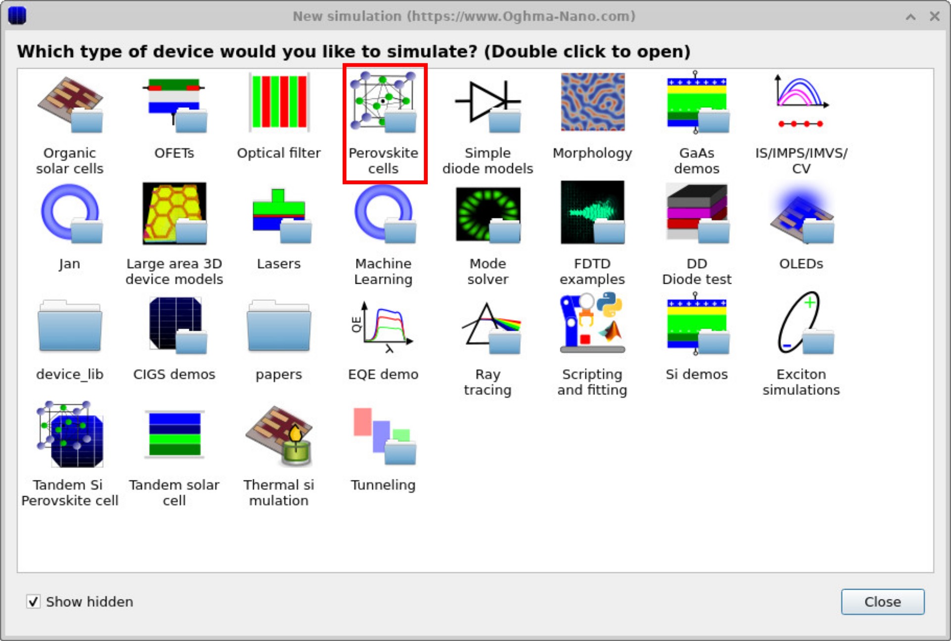
Step 1: Making a new simulation

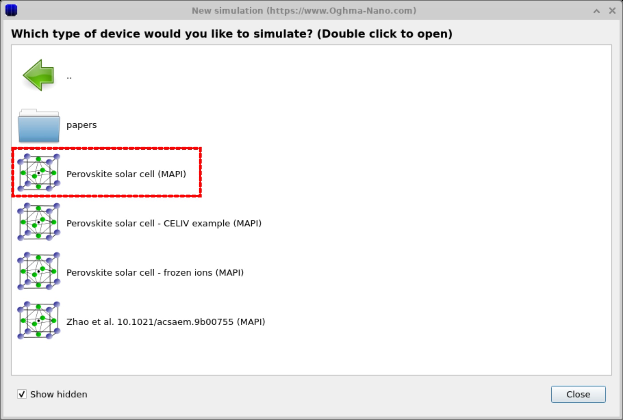
Double-click the Perovskite cells category in the new simulation window (??), then choose Perovskite solar cell (MAPI) (??) and save the project to disk. Although this tutorial uses the MAPI example, the Suns–Voc procedure works for any solar cell because it simply varies the light intensity and records the resulting V_oc.

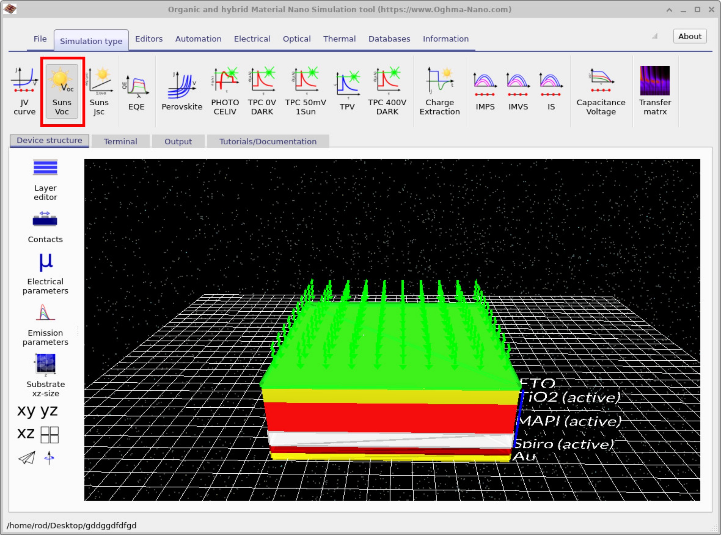
OghmaNano New simulation window with many categories; Perovskite cells folder highlighted as the target for this tutorial. — In the *New simulation* window, choose **Perovskite cells**.

Perovskite cells examples list with ‘Perovskite solar cell (MAPI)’ highlighted. — Select **Perovskite solar cell (MAPI)** and save the project to disk.

Step 2: Selecting the simulation mode

After saving, the main simulation window opens. Switch the simulator into Suns–Voc mode by going to Simulation type and clicking the Suns–Voc button—make sure the button appears pressed (??). When you run the simulation in this mode, it generates a Suns–Voc curve.

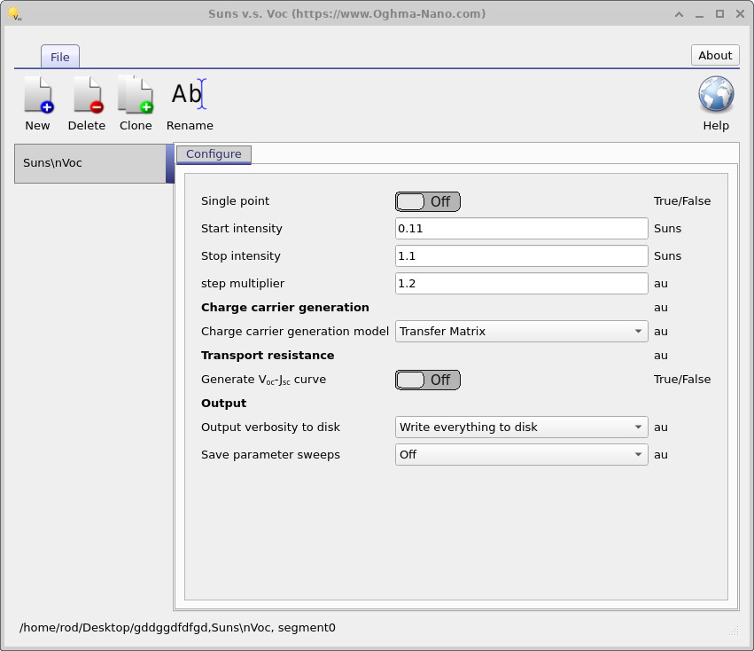
To configure the Suns–Voc experiment, open the Editors ribbon and select Suns–Voc (not shown in the ribbon here). This opens the configuration window (??), where you can specify the start intensity, stop intensity (in Suns), and the step multiplier. The step multiplier (e.g. 1.2) increases the light intensity by a fixed factor at each step, effectively sampling the curve on a logarithmic scale, which is well suited for Suns–Voc analysis. In this example the stop intensity is set to 1.1 Suns (a relatively low value, since simulations often extend to around 10 Suns) and the start intensity is slightly high, but the default values are usually adequate for most cases.

Main OghmaNano window showing a perovskite device; the Simulation type ribbon includes a Suns-Voc button to select the correct mode. — In the main window, under *Simulation type*, click **Suns-Voc** to enter the correct mode.

Suns–Voc configuration panel with start/stop intensity and step settings. — Adjust the *Suns–Voc* settings (e.g., start/stop intensity and step multiplier) as required, then run the simulation.

Step 3: Looking at the results

Once settings are confirmed, return to the main window and click Play (or press F9). When the run completes, open the Output tab (??) and locate suns_voc.csv. Opening it produces the Suns vs. V_oc plot (??).

Output tab after running the simulation showing generated files including suns_voc.csv. — After the run, open the *Output* tab and locate `suns_voc.csv`.

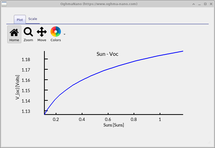
Suns–Voc plot showing open-circuit voltage (Voc) versus illumination intensity (Suns). — Opening `suns_voc.csv` displays the **Suns vs. Voc** curve.

This completes the basic Suns–Voc simulation. You have seen how to set up a perovskite solar cell, switch the simulator into Suns–Voc mode, and generate the characteristic curve. At this stage you are encouraged to experiment with the simulation options: small changes in the electrical parameters can have a large effect on the shape and slope of the Suns–Voc curve, just as they do in real experimental data. Exploring these settings will give you deeper intuition about what Suns–Voc can reveal about recombination in your devices.

📚 Homework tasks:

Task 1: Open the Electrical parameter editor from the main window. Locate the Shockley–Read–Hall (SRH) trap parameters and switch them off. Rerun the Suns–Voc simulation and observe how the slope of the curve changes.

Expected result

With traps disabled, the ideality factor should move closer to n ≈ 1, producing a straighter curve consistent with band-to-band recombination.
Task 2: Turn the SRH traps back on and increase their density by an order of magnitude. Run the simulation again and compare with the trap-free case.

Expected result

With higher trap density, the Suns–Voc curve becomes steeper at low–to–moderate light levels, corresponding to an effective ideality factor nearer to n ≈ 2. This highlights how traps increase recombination losses and alter the diagnostic value of Suns–Voc.

📈 Advanced: How to analyse your experimental Suns–Voc curve — click here to expand

Goal; From a plot of open-circuit voltage V_oc versus illumination (Suns), the main objective is to extract the ideality factor n and estimate the dark saturation current J₀. These two quantities reveal which recombination processes dominate in the device and how severe they are.

What you need; the data used to draw your Suns–Voc curve (pairs of Suns, Voc), usually saved in suns_voc.csv. We also assume room temperature (≈300 K), where k_BT/q is about 25.85 mV.

Step 1 — Prepare a semi-log plot; plot V_oc against the natural logarithm of intensity, ln(Suns). In the ideal Suns–Voc region, the curve becomes close to a straight line whose slope is set by the diode ideality factor:

\[ \text{slope} \;=\; \frac{\Delta V_{\text{oc}}}{\Delta \ln(\text{Suns})} \;\;\Rightarrow\;\; n \;=\; \frac{q}{k_\mathrm{B}T}\,\frac{\Delta V_{\text{oc}}}{\Delta \ln(\text{Suns})}. \]

A practical approach is to fit a straight line to the central part of the data (typically 0.2–0.8 Suns) and to avoid very low or very high intensities where leakage, shunt effects, or series resistance distort the curve.

Step 2 — Read off the ideality factor; at 300 K, k_BT/q is about 25.85 mV. If the slope corresponds to n ≈ 1, recombination is dominated by band-to-band processes such as radiative or surface recombination. If n ≈ 2, then trap-assisted (Shockley–Read–Hall) recombination dominates. If n falls between 1 and 2, both channels may be contributing, or the regime may vary with light intensity.

Step 3 — Estimate the dark saturation current; the Suns–Voc relation under open circuit is

\[ V_\mathrm{oc} \;=\; \frac{n k_\mathrm{B}T}{q}\; \ln\!\left(\frac{J_\mathrm{ph}}{J_0}+1\right) \quad\Rightarrow\quad J_0 \;\approx\; J_\mathrm{ph}\,\exp\!\left(-\frac{q V_\mathrm{oc}}{n k_\mathrm{B}T}\right). \]

A convenient choice is to evaluate this around 1 Sun, since the photocurrent at this point is close to the short-circuit current density, J_sc. If J_sc is not known, relative J₀ values can still be compared between devices using Suns as a proxy for the photocurrent.

What to look for on the curve; at very low Suns, downward curvature usually indicates shunt or contact leakage and should be ignored for fitting. At high Suns, a flattening trend points to series resistance or high-order recombination such as Auger processes, which should also be excluded. If the slope itself changes gradually with Suns, this often signals a transition between recombination regimes, for example trap-filling effects.

Quick checklist; plot Voc vs ln(Suns) and fit the straight-line region; calculate n from the slope using the relation above; and with n in hand, estimate J₀ around 1 Sun.

👉 Next step: Now continue to Suns-Jsc.