S-Plane Tutorial (Part A): Automated Parameter Scans for a Cooke Triplet

1. Introduction

In this tutorial, we will learn how to use the parameter scan tool in OghmaNano to systematically vary key lens parameters in a Cooke triplet, such as surface curvature and element thickness, and analyse the resulting changes in optical performance. We will run large batches of ray-trace simulations to map how individual parameters and parameter combinations influence system behaviour, and evaluate performance using quantitative metrics including RMS spot radius, encircled energy (EE50, EE80, EE90), peak intensity, and geometric aberration measures, alongside visual inspection in the 3D ray-trace view. This workflow provides a reproducible approach to lens optimisation and sensitivity analysis, and is directly applicable to early-stage lens design, tolerance studies, and rapid exploration of design trade-offs in practical optical systems.

2. Launch the Cooke triplet simulation in OghmaNano

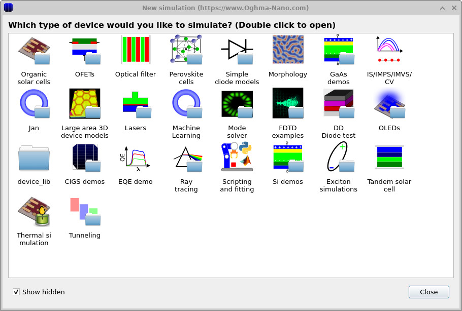
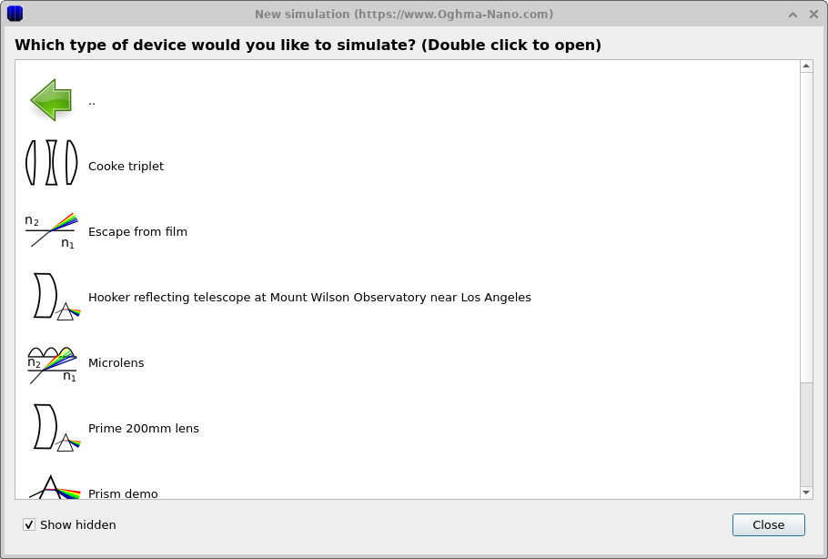
In this tutorial, we will start by launching a preconfigured Cooke triplet lens simulation. Begin by starting OghmaNano from the Windows Start menu. In the main window, click the New simulation button to open the simulation library, shown in Figures 2a–b. From the list of device categories, double-click on Ray tracing. When the S-plane optics demos appear, locate the Cooke triplet example and double-click it to open a ready-to-run lens system.

OghmaNano new simulation window listing device categories including optics and S-plane examples — The *New simulation* window provides a library of device categories. Double-click **Ray tracing** to access the S-plane optics examples.

OghmaNano S-plane examples list including Cooke triplet and other optics demos — The S-plane optics demo list. Select **Cooke triplet** to open a preconfigured lens system suitable for parameter scanning and optimisation.

💡 Tip: For best performance, save this simulation to a local drive such as C:\. In this tutorial we will be running large parameter scans, repeatedly dumping ray-trace data and 3D mesh files to disk. This generates a high volume of small read/write operations, which can become a significant bottleneck on network, USB, or cloud-synced folders (e.g. OneDrive), causing simulations to run substantially more slowly.

3. Open the Cooke triplet simulation and inspect it in the S-plane editor

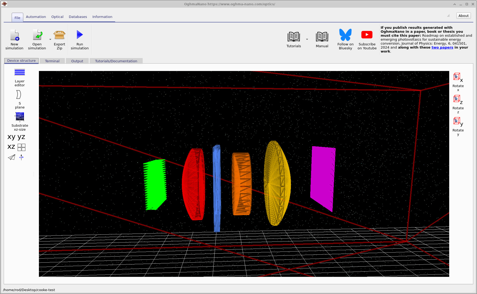
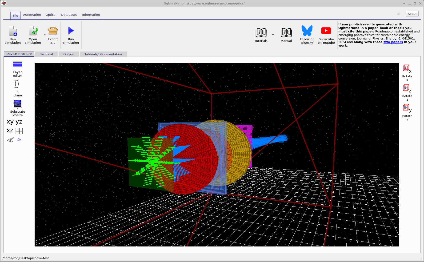
Once you have saved the Cooke triplet simulation, the main OghmaNano window will open and should look like ??. In the 3D view you can see the classical triplet layout: a green light source, the red first lens element, a blue aperture stop, the orange second lens element, the yellow third lens element, and the purple detector plane.

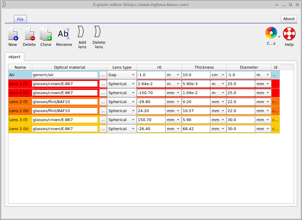
Next, click the S-plane button in the left toolbar to open the S-plane editor, shown in ??. This table lists the lens elements and their parameters (material, surface radius, thickness, diameter, etc.). In the next steps, you will use this editor to choose which parameter(s) to scan.

Main OghmaNano optics interface showing the Cooke triplet elements in 3D — The main OghmaNano optics interface after opening the *Cooke triplet* example (3D view).

S-plane editor table listing lens elements and parameters for the Cooke triplet — The S-plane editor for the Cooke triplet, listing individual lens surfaces and parameters.

As with any other simulation in OghmaNano, you can run this model by pressing the Run (play) button and inspect the results in the Output tab; however, running individual simulations will not be the focus of this tutorial.

4. Automation

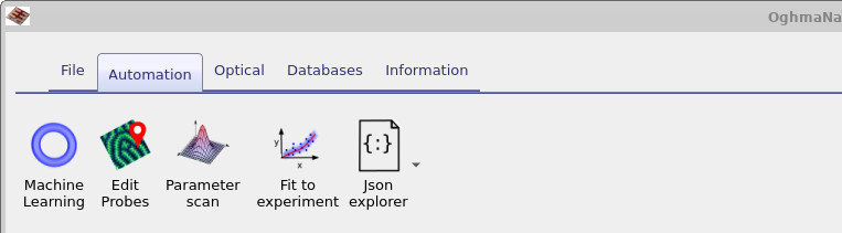
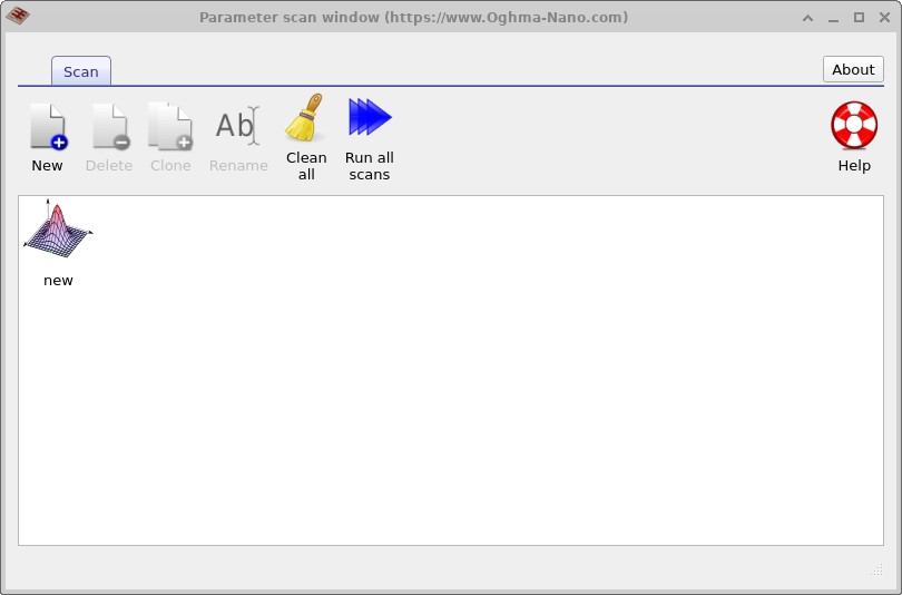
In this tutorial, we will use the Automation tools to run systematic parameter scans. These tools are accessed from the Automation ribbon in the main window (see ??). Click the Parameter scan button to open the parameter scan window (see ??). By default, you will see an entry called new; double-clicking this opens an individual parameter scan editor (see ??).

The parameter scan tool is described in more detail in the manual at https://www.oghma-nano.com/manual/parameter-scan.html. For the purposes of this tutorial, it is sufficient to know that the parameter scan window allows you to define and manage multiple independent scans using the New button, each corresponding to a different automated exploration of parameter space.

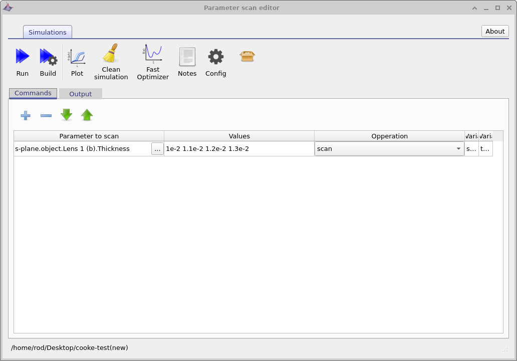
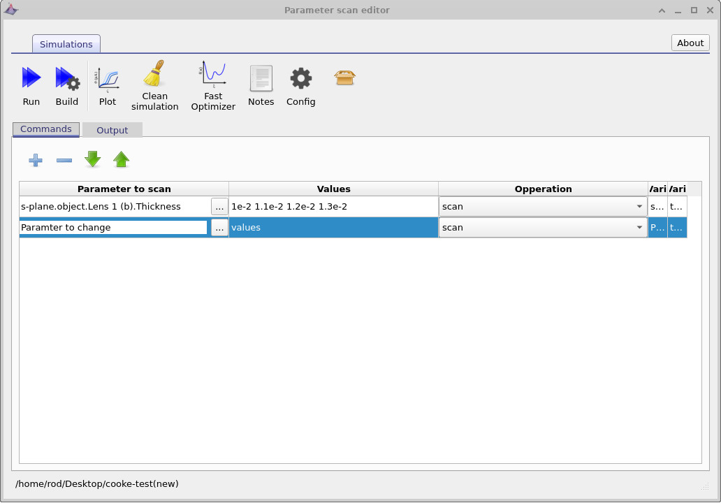
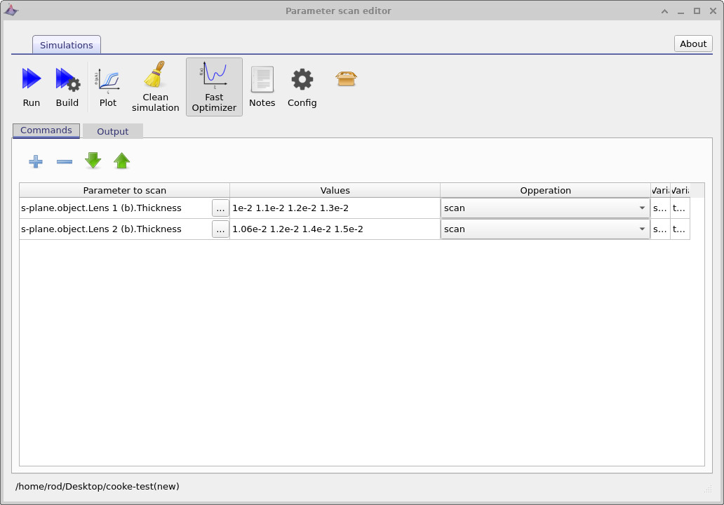
In the final figure you can see that a scan has already been configured. The variable name Splane.object.lens1.b.thickness indicates that we are scanning the thickness of the back surface of the first lens element, with the scan values specified explicitly in metres.

It is important to note that OghmaNano represents a full three-dimensional optical world. The S-plane parameter editor, while it appears similar to a conventional 2D S-plane ray-tracing interface, is in fact a derived representation of this underlying 3D geometry. All S-plane parameters are therefore virtual or derived quantities computed from the 3D model. When performing a parameter scan, you are scanning these derived S-plane parameters, which are then consistently mapped back onto the full 3D optical system during ray tracing.

Automation ribbon showing parameter scan tools — The Automation ribbon, providing access to parameter scans and batch tools.

Parameter scan window listing scan configurations — The parameter scan window listing available scan configurations.

Parameter scan editor showing scan variables and values — The parameter scan editor showing a scan over the derived S-plane lens thickness parameter.

For this task, we are going to add an additional scan line so that we scan parameters on more than one lens element. Click the plus button in the parameter scan editor to create a new scan row, as shown in ??. This adds a new line to the table with the columns Parameter to change, Values, and Operation. We will use this second row to define an additional scan, allowing multiple lens parameters to be varied in the same automated run.

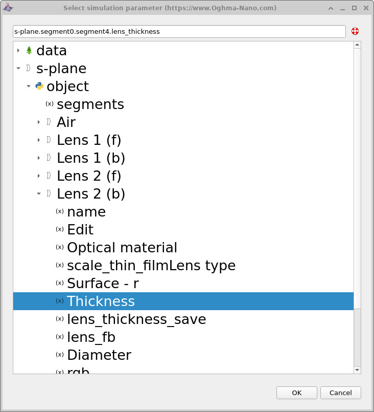
It is very important to ensure that the correct scan row is selected before editing it. Click on the new row so that it is highlighted, then click the three dots button to choose a parameter. This opens the parameter selection dialog, shown in ??. Navigate through object → Lens 2 (b) and select Thickness, which corresponds to the back-surface thickness of the second lens element. Once selected, click OK.

After configuring both scan rows, the parameter scan window should look like the final configuration shown in ??. At this point, the scan is set up to vary the thickness of two different lens elements simultaneously during the automated run.

Parameter scan editor with a newly added scan row highlighted — Adding a new scan row using the plus button.

Select simulation parameter dialog highlighting Thickness of Lens 2 back surface — Selecting the back-surface *Thickness* parameter for the second lens.

Final parameter scan window with two lens thickness scans configured — The fully configured parameter scan with two lens thickness parameters defined.

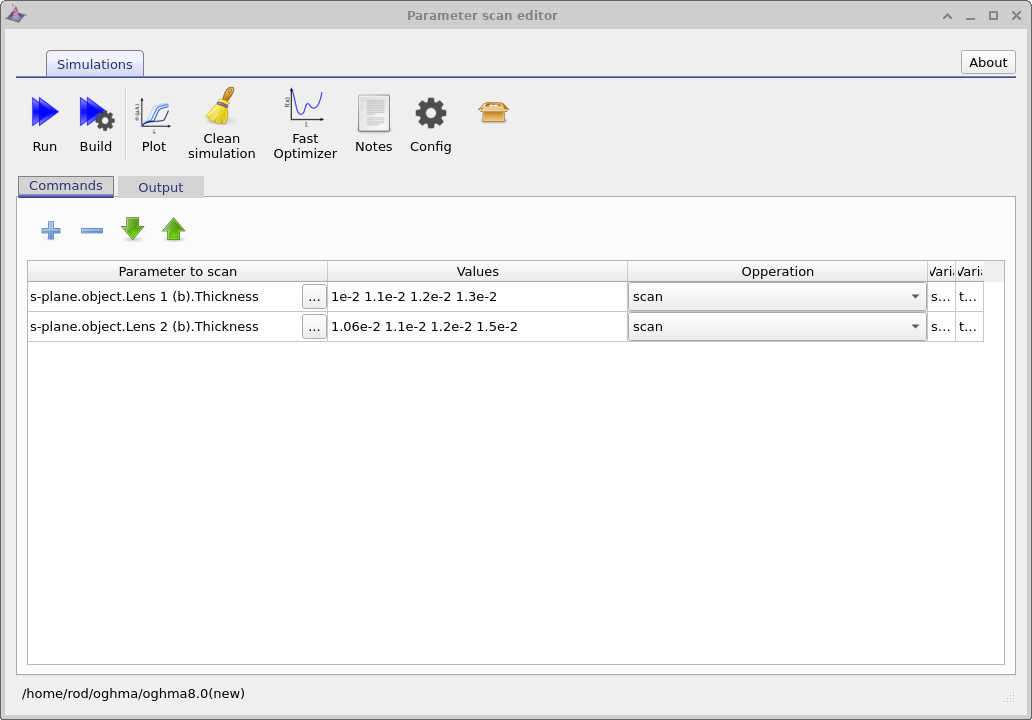
Once the parameter scan has been configured as shown in ??, click the Run button. This will execute all simulations defined by the scan. In this case, OghmaNano will run through all combinations of the scan parameters: for each value in the first scan row, it will execute all values defined in the second scan row. The result is a full exploration of all parameter permutations of the optical system.

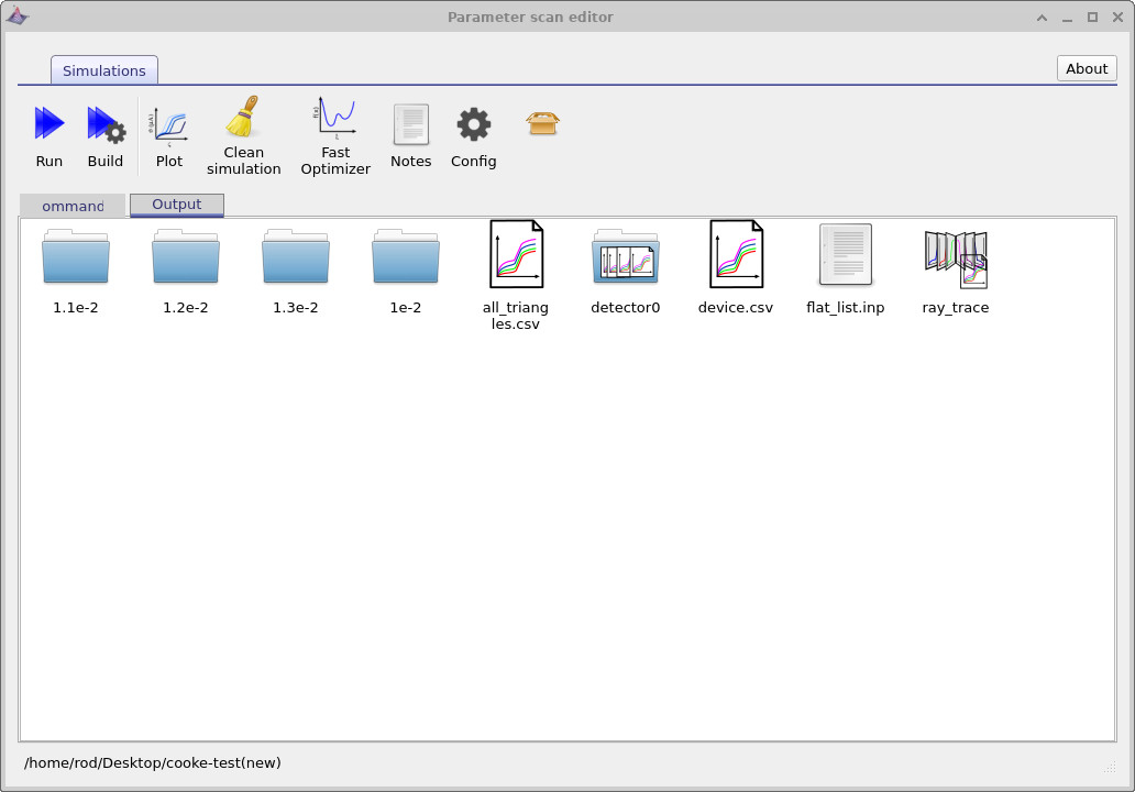
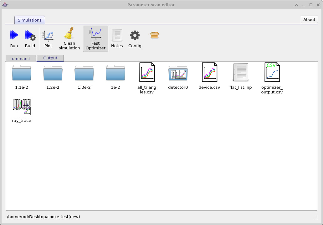
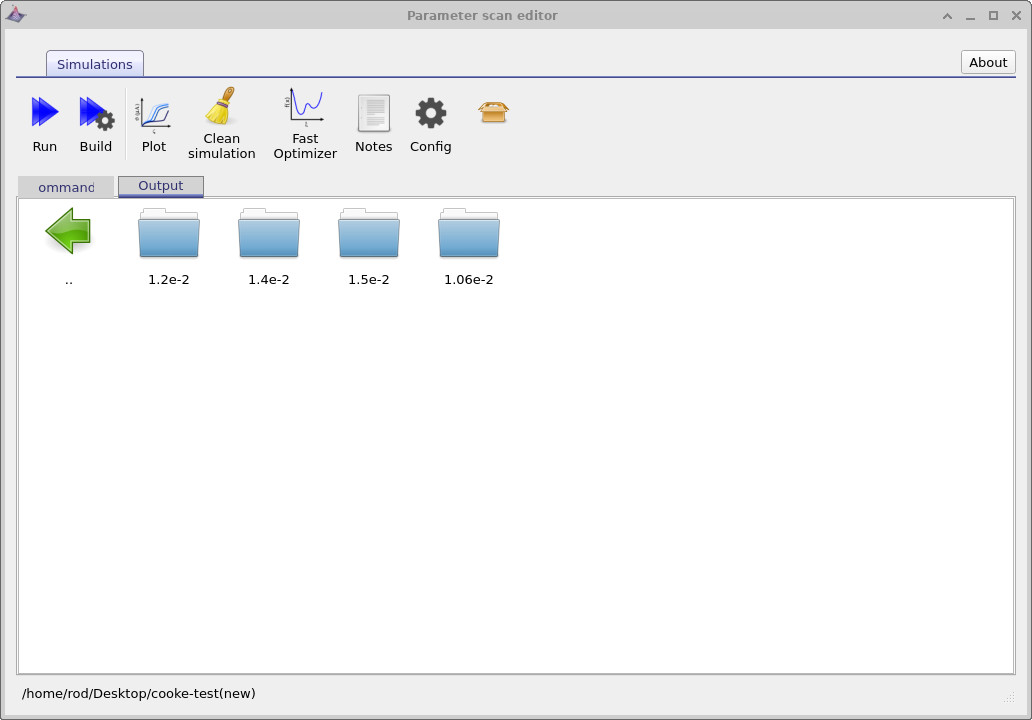
When the scan has finished, switch to the Output tab, shown in ??. The output is organised as a directory tree reflecting the scanned parameters. At the top level, the folders labelled 1.1e-2, 1.2e-2, 1.3e-2, and 1e-2 correspond to the values of the first parameter that was scanned. Navigating into one of these directories reveals subdirectories corresponding to the values of the second scan parameter, as shown in ??.

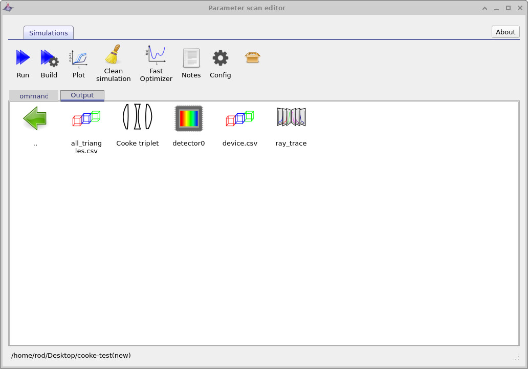
Each leaf directory represents an individual simulation run, equivalent to a single manually executed simulation. Inside these directories you will find files such as device.csv, which contains the triangulated 3D geometry of the optical system, and the ray_trace output, which stores the traced rays for that specific parameter combination. These can be visualised directly, as shown in ?? and ??. This allows you to inspect and analyse the behaviour of individual simulations corresponding to specific points in the scanned parameter space.

Parameter scan output directory showing top-level parameter folders — Running the parameter scan generates a directory tree organised by the scanned parameters.

Output tab showing parameter scan results — The *Output* tab after the scan has completed.

Nested parameter scan directories showing second parameter values — Subdirectories corresponding to the second scanned parameter.

3D device geometry from a single parameter scan simulation — Visualisation of the 3D device geometry for a single scan point.

Ray-trace visualisation for a single parameter scan simulation — Ray-trace output corresponding to the same parameter combination.

In the scan output directory you will notice several items with a multiple-curves icon. These represent a special type of scan-generated file: they are not single data files, but collections of links to the data produced across the full parameter-scan tree. For example, all_triangles.csv links to every triangulated mesh generated for all scan points, while ray_trace links to all ray-trace outputs produced during the scan.

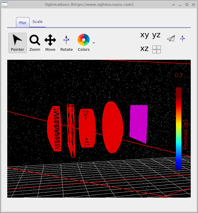
If you double-click all_triangles.csv, the mesh viewer opens (see ??). Using the slider at the bottom of the window, you can step through the individual simulations that were generated. As you move through the slider, the lens geometry updates to reflect the current parameter combination, and the active simulation path is shown at the bottom of the window. In the example shown, the path indicates the parameter combination 1.2e-2 / 1.4e-2, corresponding to the two scanned lens-thickness values (in metres).

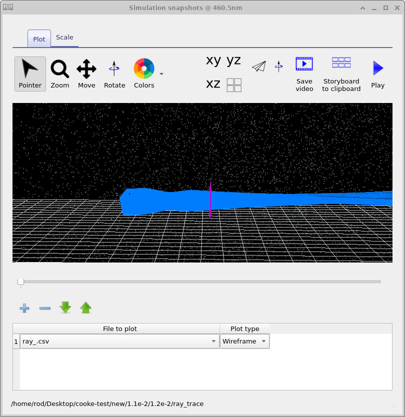
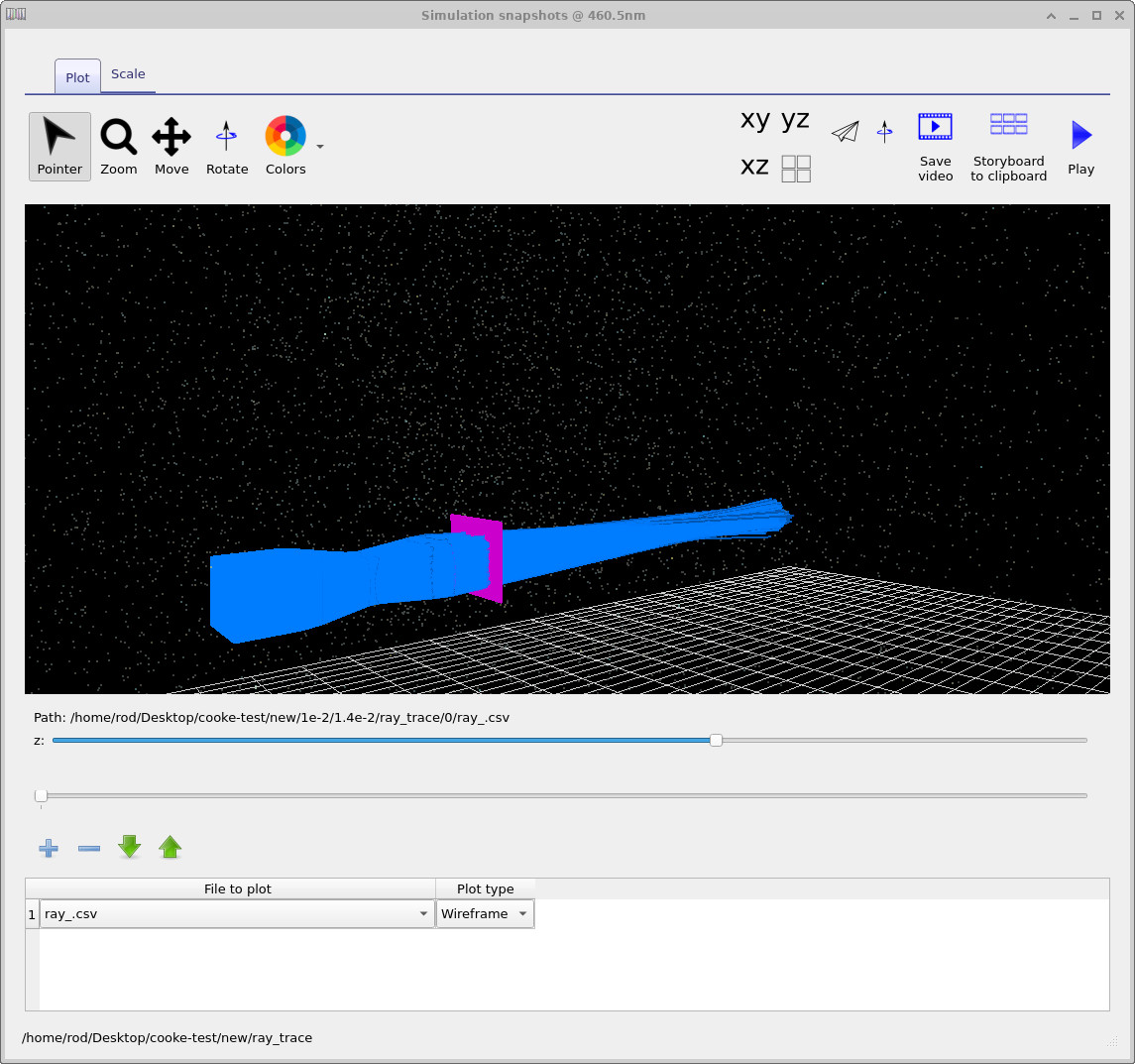
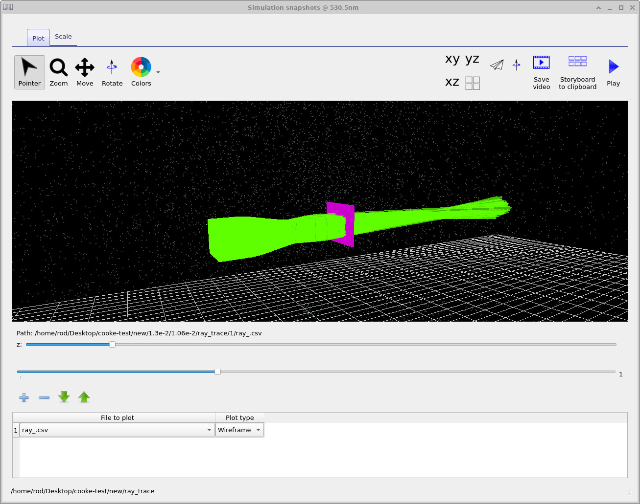
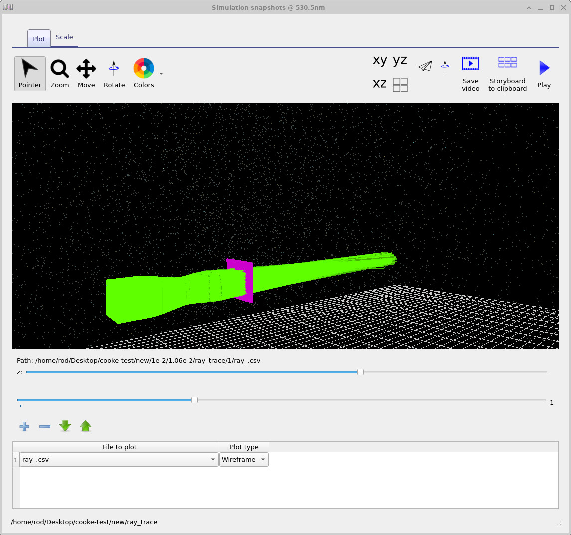
Similarly, double-clicking ray_trace opens the ray-trace viewer (see ??). This viewer typically provides two sliders: the upper slider steps through the different simulations in the scan tree, while the lower slider steps through wavelength. This makes it possible to inspect how ray paths evolve both across parameter space and across wavelength. A second example, shown in ??, illustrates the same scan viewed at a different wavelength range. If nothing is visible initially, you may need to click the plus button in the plot table to add a file to plot.

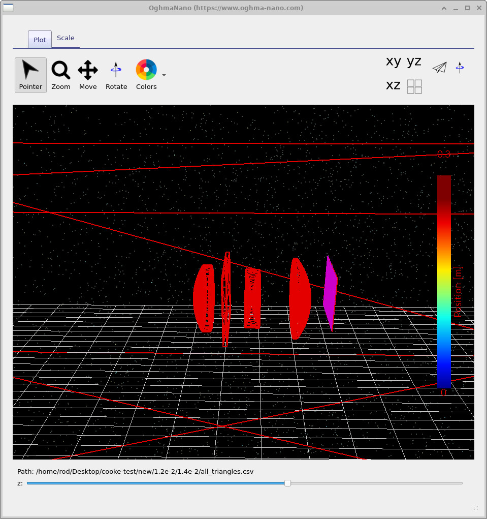
Viewer showing all triangulated meshes generated during the parameter scan — Viewing `all_triangles.csv`: stepping through the triangulated meshes generated across the full parameter scan.

Ray-trace viewer stepping through scan points and wavelength — Ray-trace viewer showing rays for different scan points and wavelengths using the two sliders.

Ray-trace viewer showing the same scan at a different wavelength range — The same ray-trace scan viewed at a different wavelength range.

As a further example of these scan meta-files, navigate into the detector0 output folder and double-click it (see ??). You will again see multiple-curves items corresponding to different detector outputs. If you double-click detector_efficiency0.csv, OghmaNano will open the plot shown in ??. This plot shows how much light the system transmits (as a percentage) as a function of wavelength, with one curve for each lens geometry explored in the parameter scan. Note that this example uses only three optical mesh points, so each curve contains only three wavelength samples.

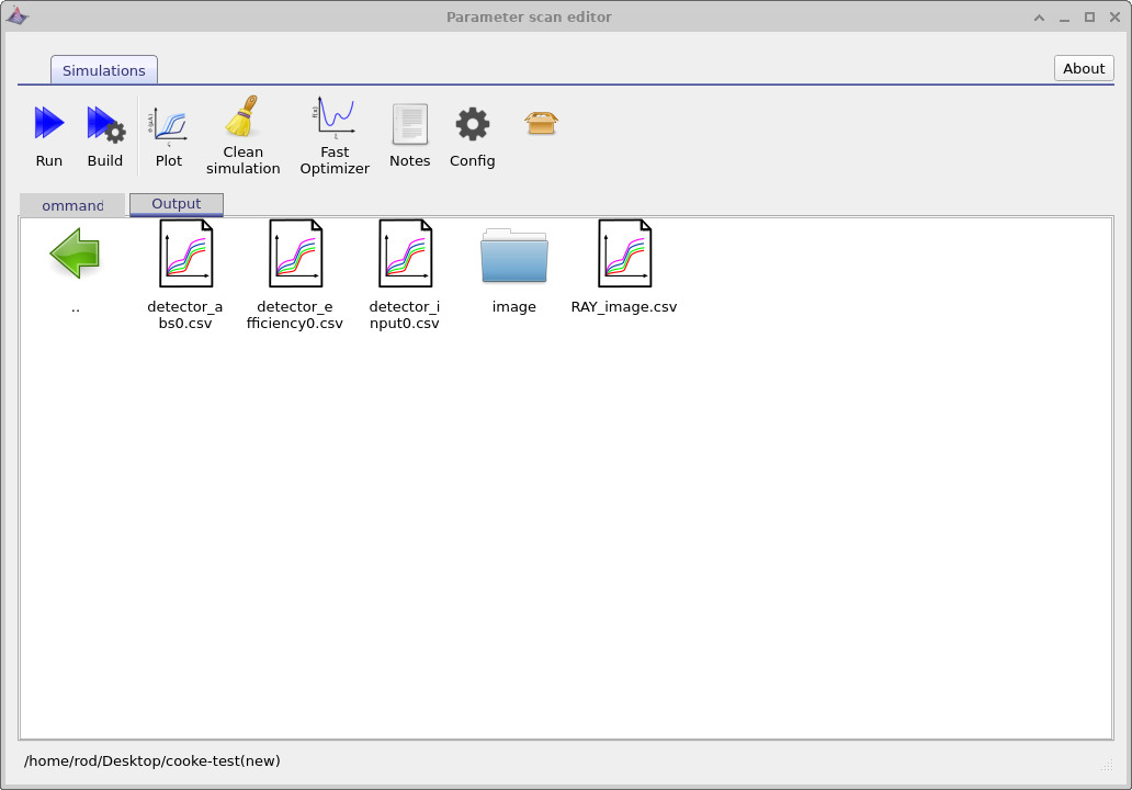
Detector output folder showing scan meta-files for different detector outputs — The `detector0` output folder containing scan meta-files for detector outputs (e.g. efficiency and input).

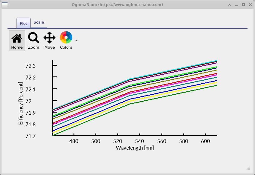
Detector efficiency plot versus wavelength showing multiple curves for different scan points — `detector_efficiency0.csv` plotted versus wavelength: one curve per lens geometry explored in the scan.

5. Optimizer

In the previous section, we used the parameter scan tool to brute-force generate a large number of simulations that we could inspect directly by looking at ray paths, geometries, and detector outputs. While this is very useful for building physical intuition, it also generates a large number of files, consumes significant disk space, and slows the overall simulation workflow. In many cases, you instead want a fast sweep through parameter space that focuses on quantitative performance metrics rather than full output data.

To do this, we use the optimizer. Return to the parameter scan editor (see ??) and click the Fast optimizer button. This mode disables the generation of detailed output files (ray traces, meshes, etc.) while still running the underlying simulations and collecting statistical metrics. Importantly, any output files generated by earlier scans are left untouched and can still be inspected; the optimizer simply avoids creating new ones.

After enabling the fast optimizer, rerun the simulation. When it completes, open the Output tab (see ??). You will see a new file called optimizer_output.csv. Unlike the full scan, no new directory tree is created: the primary result of the optimizer is this single CSV file containing the aggregated performance data.

Parameter scan editor with the Fast optimizer button highlighted — Enabling the *Fast optimizer* in the parameter scan editor.

Output tab showing optimizer_output.csv — The `optimizer_output.csv` file produced by the fast optimizer.

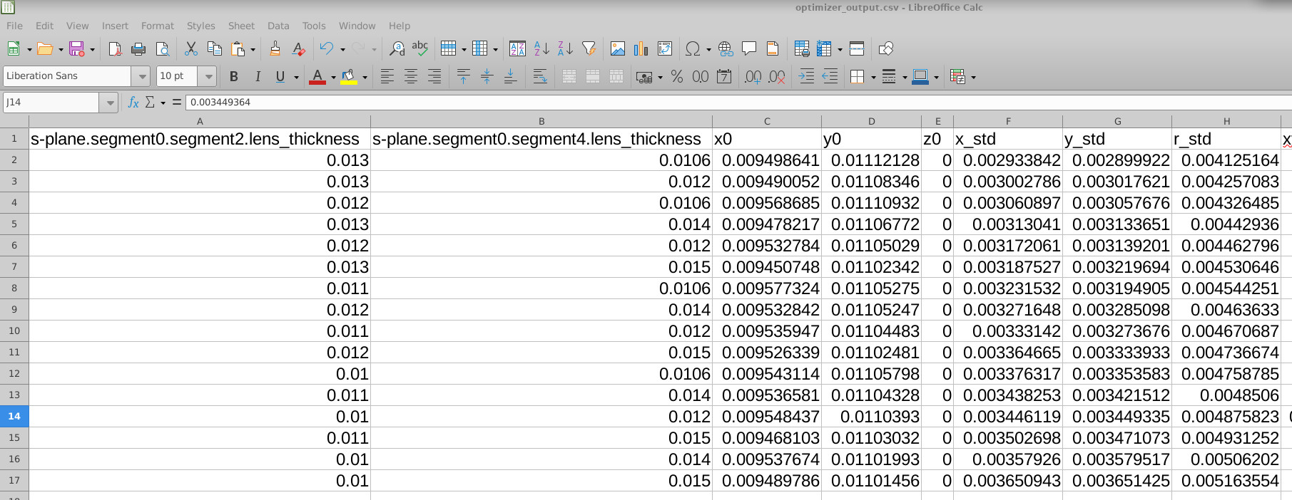
Double-click optimizer_output.csv and open it in your preferred spreadsheet program (Excel, LibreOffice, or any tool that can read CSV files). The contents are shown in ??. The first columns list the parameters that were scanned (in this case the S-plane lens thicknesses), followed by a range of quantitative performance metrics extracted from each simulation.

These metrics include the standard deviation of the spot position in x and y, the standard deviation of the spot radius (r_std), the major and minor axes of the spot distribution (sigma_major, sigma_minor), the spot orientation angle (spot_theta), encircled-energy radii (e.g. EE50, EE80, EE90), and related goodness measures. Together, these provide a compact quantitative summary of optical performance for every point in the scanned parameter space.

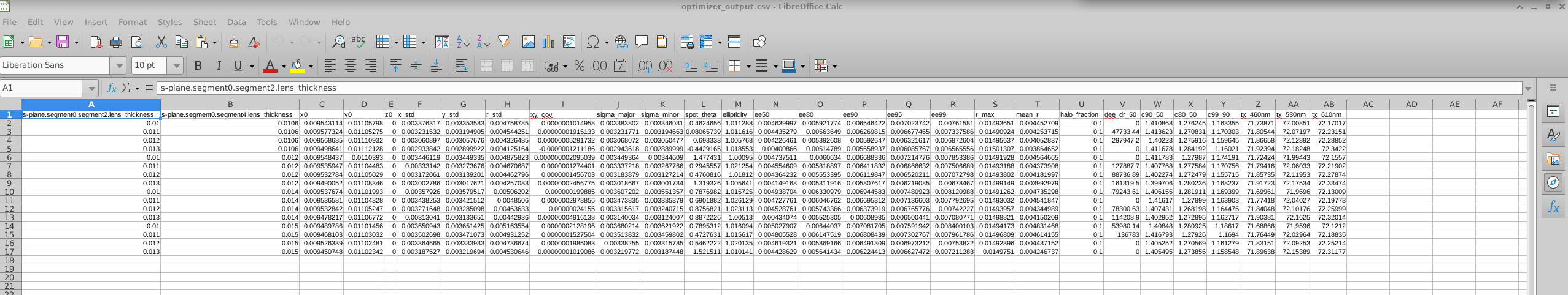
optimizer_output.csv opened in a spreadsheet showing scan parameters and performance metrics — The contents of `optimizer_output.csv`, showing scanned parameters alongside spot and efficiency metrics.

Because the data are in tabular form, you can easily sort or filter them to identify optimal designs. For example, in ?? the spreadsheet has been sorted by r_std, the standard deviation of the spot radius. From this we can immediately see which combination of lens thicknesses produces the smallest spot: in this case a first-lens thickness of 0.013 and a second-lens thickness of 0.0106.

optimizer_output.csv sorted by spot radius standard deviation — Sorting the optimizer output by *r_std* to identify the best-performing lens geometry.

6. Examining results from the optimizer

Now that we have run both the systematic parameter scan and the optimizer, we can examine the results in more detail. The optimizer allows us to quickly identify promising regions of parameter space, while the full scan lets us inspect the corresponding simulations in a more physical and visual way.

As a first step, we can return to the ray-trace outputs and locate the simulation corresponding to the minimum spot-size solution identified by the optimizer. This is shown in ??. Using the selector bars in the ray-trace viewer, you can move through the simulation tree until you reach the parameter combination that produced the smallest spot.

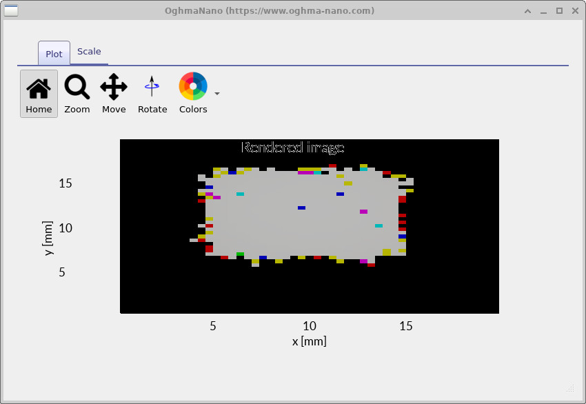
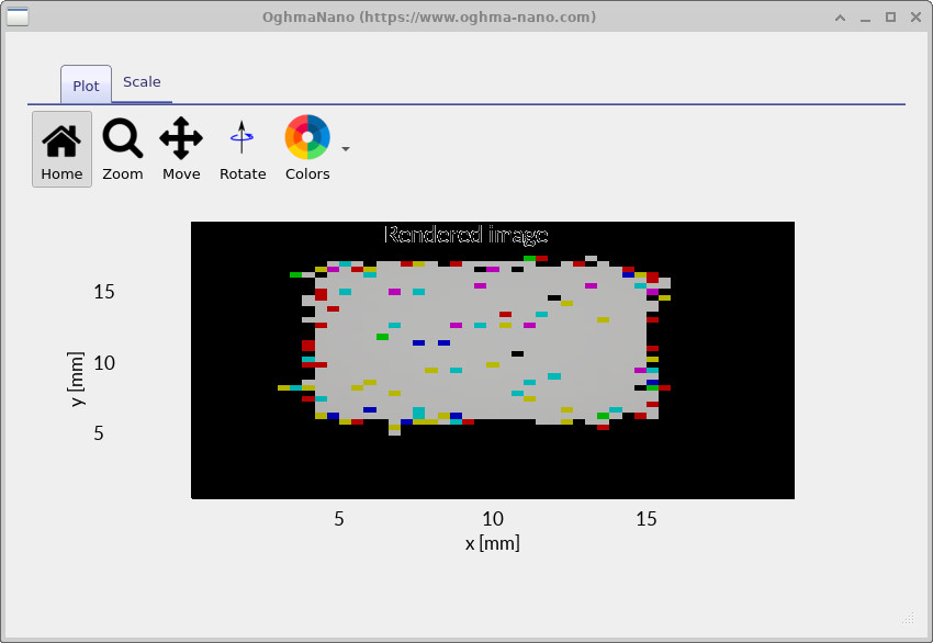
We can then dig further into the simulation tree to compare how the optical system behaves for different parameter choices. For example, ?? shows a relatively small, well-focused spot corresponding to a near-optimal design, while ?? shows a larger, less optimal spot produced by a different point in the scanned parameter space.

Ray-trace view corresponding to the minimum spot-size solution found by the optimizer — Ray-trace visualisation of the minimum spot-size solution identified by the optimizer.

Detector image showing a small, well-focused spot for an optimal lens configuration — A small, well-focused spot corresponding to a near-optimal lens configuration.

Detector image showing a larger spot for a less optimal lens configuration — A larger spot produced by a less optimal point in the scanned parameter space.

Taken together, this illustrates a typical workflow: first run the optimizer to quickly explore parameter space and identify promising regions, then disable the optimizer and perform a full scan in the region of interest. This allows you to generate detailed outputs—ray traces, geometries, and detector images—that can be inspected physically to confirm that the solution behaves as expected and meets your design goals.

7. Using alternative beam shapes to speed up simulations

In the previous sections, we used a square beam to run both the parameter scan and the optimizer. While this is a sensible default, a square beam contains a large number of rays and can significantly slow down simulations. In many cases, you do not need a full square-beam profile to understand system behaviour, and simpler beam shapes are sufficient.

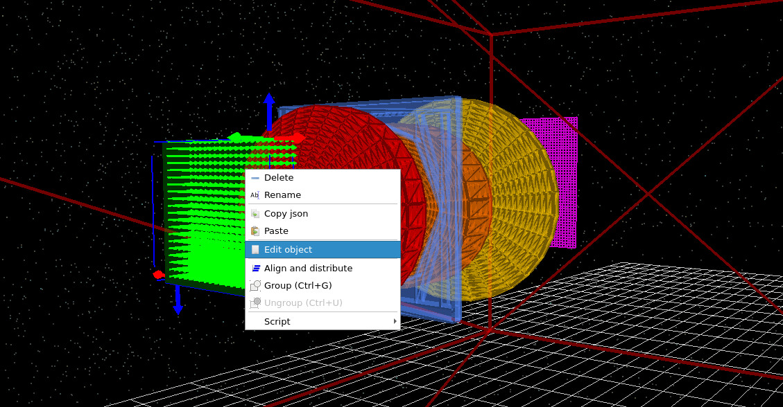
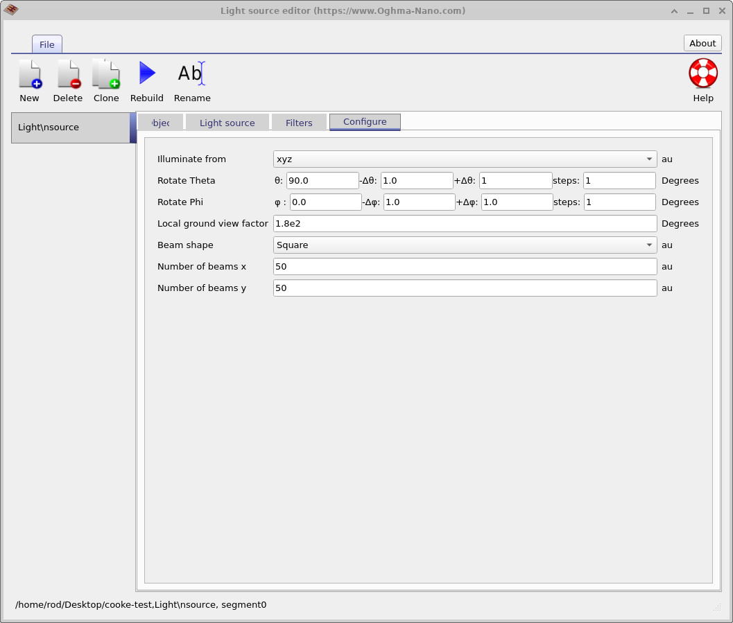
To change the beam shape, right-click on the light source in the 3D view, as shown in ??, and select Edit object. In the light source editor, navigate to the Configure tab (see ??) and change the Beam shape from Square to Star. The resulting ray pattern is shown in ??.

If you now rerun the optimizer, you will notice that the simulation completes more quickly. This is because the star beam uses far fewer rays than a full square beam, while still sampling the optical system effectively. There is also an option to use a Cross beam shape, which is useful for examining astigmatism independently along the two principal axes and reduces the computational cost even further. These alternative beam shapes are therefore a practical way to speed up exploratory scans and optimisation runs.

Right-click context menu on the light source showing Edit object — Right-click the light source and select *Edit object*.

Light source editor showing beam shape configuration — Changing the beam shape in the light source *Configure* tab.

Star-shaped beam pattern in the ray-trace view — A star-shaped beam uses fewer rays while still sampling the optical system.

8. Summary

In this tutorial, we explored how to use the S-plane optics workflow in OghmaNano to systematically investigate and optimise a classical Cooke triplet lens system. Starting from a predefined example, we learned how the S-plane editor provides a compact, ray-optics–friendly view of a fully three-dimensional optical system, with all S-plane parameters derived consistently from the underlying 3D geometry.

We then used the parameter scan tool to perform brute-force exploration of lens design space by varying multiple lens parameters simultaneously and running all permutations of the resulting optical systems. This allowed us to inspect individual simulations in detail, visualise ray paths and geometries, and build physical intuition about how changes in lens thickness and spacing affect system performance.

To enable faster exploration, we introduced the fast optimizer, which disables heavy output generation while collating quantitative performance metrics into a single CSV file. By analysing these metrics—such as RMS spot size, encircled energy, and spot ellipticity—we were able to identify optimal parameter combinations efficiently and link them back to specific lens geometries.

Finally, we showed how alternative beam shapes (star and cross) can dramatically reduce computational cost while still capturing key optical behaviour, making them well suited for optimisation and exploratory scans.

Together, these tools form a practical and reproducible optimisation loop: use the optimizer to locate promising regions of parameter space, then switch to full parameter scans with detailed output to inspect ray behaviour and validate physical performance. This workflow scales naturally from simple lens systems to more complex optical designs and provides a robust foundation for systematic lens optimisation in OghmaNano.