Quick start: Solar Spectrum Generator overview

In this quick start we use OghmaNano’s Solar Spectrum Generator to simulate solar spectral irradiance at the Earth’s surface. The tool outputs the standard AM1.5G solar spectrum alongside calculated global, direct, and diffuse irradiance components. These spectra can be exported and applied directly in optical or photovoltaic device simulations.

1. Background:

The generator is based on the Simple Solar Spectral Model for Direct and Diffuse Irradiance on Horizontal and Tilted Planes at the Earth's Surface for Cloudless Atmospheres by Bird and Riordan (1986), published in the Journal of Applied Meteorology and Climatology (link). This model is widely used for solar irradiance modeling in photovoltaics and atmospheric science.

The spectrum is computed by accounting for major atmospheric processes: Rayleigh scattering, absorption by ozone, gases, and water vapour, plus attenuation by aerosols and particulates. Input parameters include time of day, date, latitude, altitude, and atmospheric conditions such as pressure, aerosol optical depth, and water vapour content.

These controls let you explore how solar spectra vary with environment. For example, lower sun angles (morning/evening) increase air mass and red-shift the spectrum, while high water vapour content enhances near-infrared absorption bands. Increased aerosols or pollution reduce direct irradiance and boost the diffuse component — spectra for a polluted city like Beijing look very different to those for London or a clean, high-altitude site.

Generating and comparing spectra under different conditions helps demonstrate how atmospheric and environmental factors influence device illumination. For benchmarking, the standard AM1.5G spectrum is included, which integrates to ~1000 W m⁻² under standard test conditions.

2. Getting started:

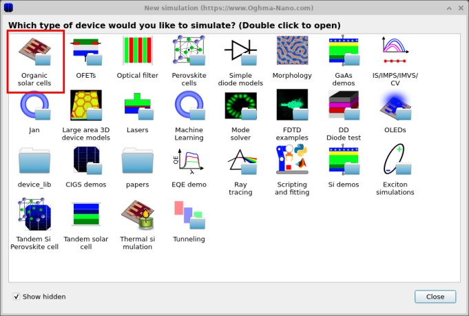
To begin, open the New simulation window from the File ribbon in the main menu. For this tutorial we will select an Organic solar cell example (see ??). You can choose any of the available devices — the solar spectra generated are independent of the device type — but organic solar cells make a useful demonstration case (see ??).

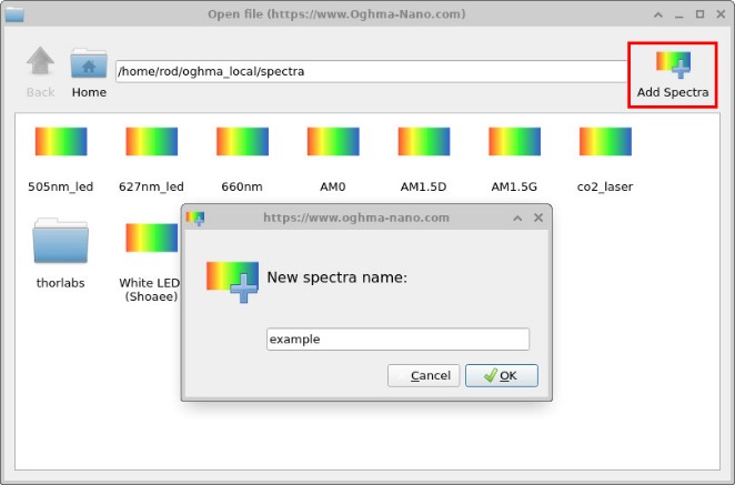
Once the simulation has been created, go to the Optical ribbon and click the Optical database icon (see ??). This will open the database where solar spectra can be viewed, generated, and imported.

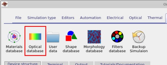
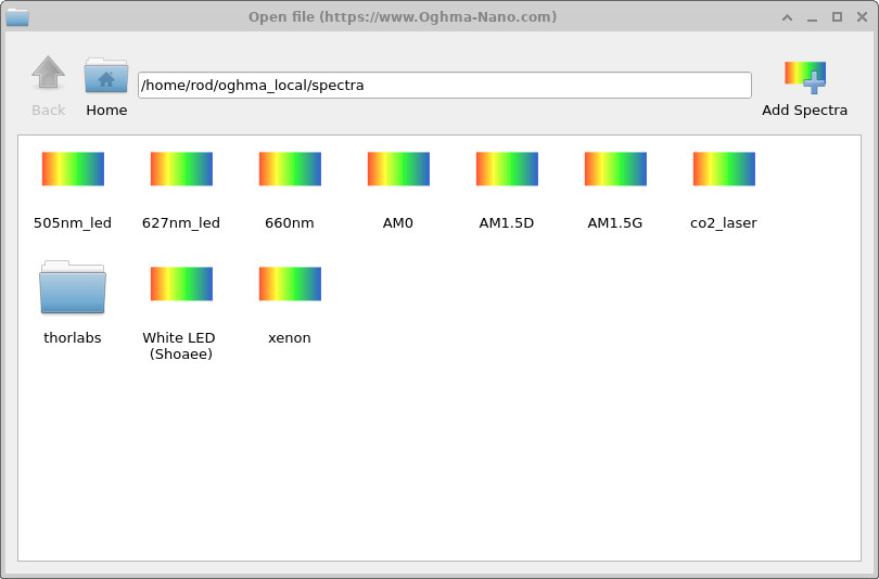
Once you have selected the Optical database item, the database window will open (see ??). Here you can see existing spectra such as AM1.5G, AM0, LEDs, and lasers. To create a new entry, click the Add Spectra button on the right-hand side. This opens a dialog (see ??) where you can enter a name for the new spectrum. In this example we will call it Example.

After confirming, a new icon labelled Example will appear in the database window. Double-clicking this new item will open the Optical Spectrum Editor (see ??), where you can view, edit, or import spectral data.

3. Generating spectra with the Solar Spectrum Generator

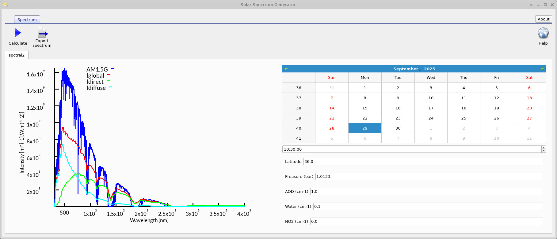
From the Optical Spectrum Editor (??), click Solar spectrum generator. This opens the generator shown in ??, ??, and ??. The tool implements the model described by Bird and Riordan (1986), Simple Solar Spectral Model for Direct and Diffuse Irradiance on Horizontal and Tilted Planes at the Earth's Surface for Cloudless Atmospheres (link), to compute AM1.5G alongside calculated global, direct, and diffuse components under user-defined conditions.

Time of day — Sets the solar hour. As the sun moves lower (morning/evening), the solar zenith angle increases, path length through the atmosphere grows (higher air mass), and UV/visible attenuation rises; the spectrum tends to red-shift slightly and the diffuse fraction increases.

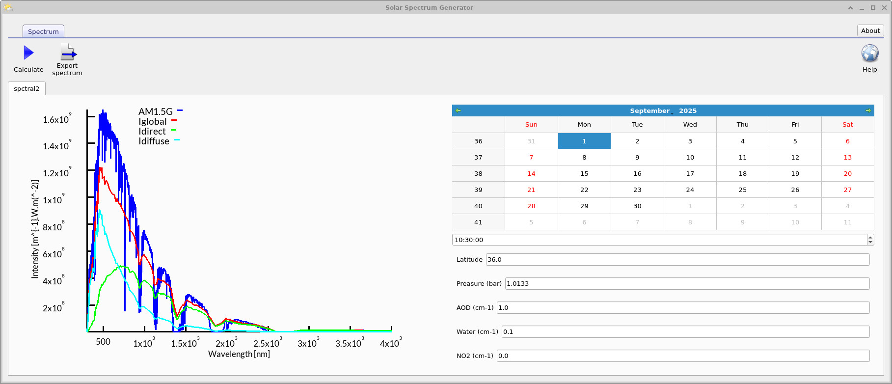
Date (day of year) — Controls seasonal geometry (declination). Summer dates yield higher solar elevation at a given location, increasing direct irradiance; winter dates reduce it. This explains the differences seen between ?? and ??.

Latitude — Sets observer location. Lower latitudes generally experience higher peak solar elevation and thus lower air mass; high latitudes see more atmospheric traversal, boosting Rayleigh and aerosol effects and reducing the direct component.

Pressure — Approximates altitude/meteorology. Lower pressure (high altitude) reduces molecular density and Rayleigh scattering, increasing short-wavelength transmittance; higher pressure does the reverse.

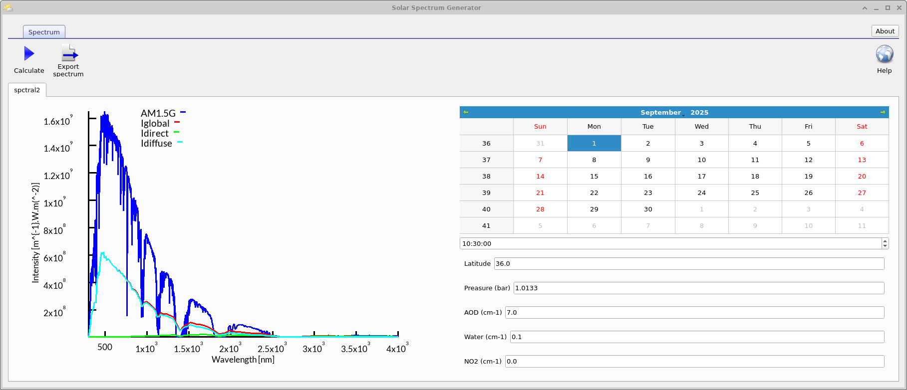
Aerosol optical depth (AOD) — Represents particulate loading (haze/pollution). Larger AOD strengthens aerosol extinction, suppressing the direct beam and transferring energy to the diffuse component. Compare the clean case with the polluted case in ??.

Water content — Sets precipitable water vapour. Increasing this deepens near-IR absorption bands (e.g., around 940 nm and beyond), reducing IR irradiance while leaving most of the visible less affected.

Adjust these controls to generate site- and condition-specific spectra, then export the result for use elsewhere in the simulation workflow.

4. Comparing AM1.5G, I_global, I_direct, and I_diffuse

When running the Solar Spectrum Generator, the results are plotted alongside the standard AM1.5G reference spectrum. This reference is widely used in photovoltaics as a benchmark for testing and comparing solar cell performance under "1 sun" conditions.

The generator additionally outputs three components of the solar irradiance:

• I_global: The total irradiance reaching a horizontal surface at ground level. It is the sum of I_direct and I_diffuse, and is the spectrum used in OghmaNano for the final photovoltaic device simulations.
• I_direct: The unscattered, collimated beam travelling directly from the sun’s disk to the surface. It dominates under clear skies and high sun elevation, but diminishes strongly under haze, pollution, or at high air masses (e.g., morning/evening, higher latitudes).
• I_diffuse: The scattered component arising from molecules, aerosols, and particulates in the atmosphere. It fills in the sky dome and increases in importance when the direct beam is attenuated — for example, during cloudy, hazy, or polluted conditions.

Comparison to AM1.5G: The AM1.5G spectrum is essentially a fixed standard representing I_global at an air mass of 1.5 and a tilt angle typical for mid-latitudes. In contrast, the simulated I_global, I_direct, and I_diffuse curves vary dynamically with location, season, time of day, and atmospheric conditions. Comparing them allows you to see how real-world conditions deviate from the "idealized" AM1.5G case.