FDTD light sources
Introduction
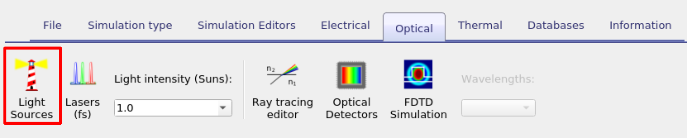
In OghmaNano, all illumination is provided by light sources. The general Light Source Editor, including spectral sources, filters, and orientation options is described in detail on the main light source page (Light sources - setup and parameters). The present page focuses specifically on how light sources are used within the finite-difference time-domain (FDTD) solver. The Light Source Editor can be accessed from the Optical ribbon in the main window (see Figure ??). This page explains how to configure time-domain excitation sources in an FDTD simulation, including waveform selection, injection mode, phase control, temporal gating, and windowing.
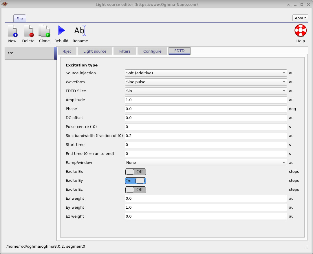
Any light source defined in OghmaNano can be used in the FDTD model. For FDTD simulations, the source is configured in the FDTD tab of the Light Source Editor (see Figure ??). This tab defines how the electric field is injected into the computational grid, including the excitation waveform, amplitude, phase, temporal gating, and the selected field components \(E_x\), \(E_y\), and \(E_z\).
In addition to the time-domain settings, the physical shape and position of the source are defined using the usual size and placement controls, either in the 3D device editor or within the Light Source Editor. By adjusting these spatial parameters, the excitation can be configured as a plane, line, box, or point source, directly controlling the geometry of the emitted field within the FDTD simulation. The detailed behaviour of the excitation waveform and its interaction with the FDTD grid are described in the following sections.
2. FDTD excitation
For FDTD simulations, a light source is defined as a time-domain excitation that injects electric-field components into the simulation region. The FDTD tab (??) controls the waveform \(s(t)\), its timing, and how it is applied to the field components \(E_x, E_y, E_z\) at the chosen injection surface or point set.
2.1 Waveform type
The Waveform selection defines the analytic form of the source function \(s(t)\). The available excitation types are Continuous sine (CW), Gaussian sine pulse, Ricker wavelet, and Sinc pulse.
In all cases, the injected scalar is written as
\[ s(t) = A\,u(t) + s_\mathrm{dc}, \]
where \(u(t)\) is the selected waveform, \(A\) is the Amplitude, and \(s_\mathrm{dc}\) is the DC offset. The excitation wavelength is set in the Optical Mesh Editor, with angular frequency related to wavelength by \( \omega = \dfrac{2\pi c}{\lambda} \). At each FDTD time step, the excitation produces a scalar value \(s(t)\) which is distributed to selected field components using weights \((w_x,w_y,w_z)\):
\[ \Delta E_x(t)=w_x s(t),\quad \Delta E_y(t)=w_y s(t),\quad \Delta E_z(t)=w_z s(t). \]
The Excite Ex/Ey/Ez switches define which components receive injection, or explicit weights may be provided.
| Waveform | Mathematical form \(u(t)\) | Description |
|---|---|---|
| Continuous sine (CW) | \[ u(t) = \sin(\omega t + \phi) \] | Monochromatic steady-state excitation at the carrier frequency. Used for single-frequency or steady-state simulations. |
| Gaussian sine pulse | \[ u(t)= \exp\!\left(-\frac{1}{2}\left(\frac{t-t_0}{\sigma}\right)^2\right) \sin\!\left(\omega (t-t_0)+\phi\right) \] | Sinusoidal carrier with Gaussian envelope. Shorter \(\sigma\) gives broader spectrum; longer \(\sigma\) approaches CW excitation. |
| Ricker wavelet | \[ u(t) = (1-2a^2)\exp(-a^2), \quad a=\pi f_0 (t-t_0) \] | Broadband impulse-like excitation (Mexican-hat wavelet). Compact and symmetric in time; useful for impulse-response analysis. |
| Sinc pulse | \[ u(t)= \mathrm{sinc}\!\left(2\beta f_0 (t-t_0)\right) \sin\!\left(\omega (t-t_0)+\phi\right) \] | Band-limited excitation with controllable bandwidth \(\beta\). Increasing \(\beta\) broadens spectral content. |
The DC offset \( s_{\mathrm{dc}} \) adds a constant component to the excitation. The waveform is time-gated by the Start time and End time parameters.
\[ s(t)=0 \quad t<t_{\mathrm{start}}, \qquad s(t)=0 \quad t>t_{\mathrm{end}}, \; t_{\mathrm{end}}>0 \]
If \(t_{\mathrm{end}}=0\), the source runs until the end of the simulation.
2.2 Phase
The Phase parameter introduces a phase shift in the time-domain carrier component of the excitation. The user-defined value in degrees is converted to radians via \( \phi=\phi_{\mathrm{deg}}\pi/180 \) and is applied to the oscillatory term of the selected waveform. When multiple coherent sources are present, this parameter sets the relative phase between them, allowing constructive or destructive interference to be controlled within the FDTD simulation.
2.3 Pulse centre (t0)
For pulsed waveforms, the oscillation is written in terms of
\[ \Delta t = t - t_0, \]
so that the waveform peak remains centered at the specified pulse time \(t_0\).
2.4 Source injection mode
The Injection mode controls how the source is applied to the electric field components at the injection cells.
In Soft (additive) mode, the excitation is added to the existing field values:
\[ E_\alpha(t) = E_\alpha(t) + \Delta E_\alpha(t). \]
In Hard (overwrite) mode, the field at the injection cells is set equal to the source value:
\[ E_\alpha(t) = \Delta E_\alpha(t). \]
Soft mode adds the excitation to the evolving solution, while hard mode directly enforces the source value at the injection location.
2.5 Ramp and windowing
The Ramp/window control applies a multiplicative function \( w(t) \) to the excitation waveform so that the injected signal becomes \( s(t) = A\,u(t)\,w(t) + s_{\mathrm{dc}} \). This limits the temporal support of the source and smooths its turn-on and turn-off behaviour.
Let the gated time variable be \( \tau = t - t_{\mathrm{start}} \), and let \( T \) denote the total window duration. For a finite window, the excitation is supported only for \( 0 < \tau < T \), and \( w(\tau)=0 \) outside this interval.
For a Hann window, the function is
\[ w(\tau) = \begin{cases} \dfrac{1}{2}\left(1-\cos\left(2\pi \tau/T\right)\right), & 0 < \tau < T, \\ 0, & \text{otherwise}. \end{cases} \]
The Hann window smoothly raises the signal from zero, reaches a maximum at mid-duration, and returns smoothly to zero at \( \tau = T \).
For a Blackman window, the function is
\[ w(\tau) = \begin{cases} 0.42 -0.5\cos\left(2\pi \tau/T\right) +0.08\cos\left(4\pi \tau/T\right), & 0 < \tau < T, \\ 0, & \text{otherwise}. \end{cases} \]
The Blackman window provides stronger suppression of spectral sidelobes than the Hann window, at the cost of a slightly broader main lobe.
For a Tukey window, a cosine taper is applied over a fraction \( \alpha \in [0,1] \) of the total duration. Defining the normalized time \( x=\tau/T \), the window is
\[ w(x)= \begin{cases} \dfrac{1}{2}\left(1-\cos\left(\pi x/\frac{\alpha}{2}\right)\right), & 0 < x < \frac{\alpha}{2}, \\[6pt] 1, & \frac{\alpha}{2} \le x \le 1-\frac{\alpha}{2}, \\[6pt] \dfrac{1}{2}\left(1-\cos\left(\pi (1-x)/\frac{\alpha}{2}\right)\right), & 1-\frac{\alpha}{2} < x < 1, \\[6pt] 0, & \text{otherwise}. \end{cases} \]
When \( \alpha=0 \), the Tukey window reduces to a rectangular window (no taper). When \( \alpha=1 \), it becomes equivalent to a Hann window.
Windowing is important in FDTD because abrupt truncation of a waveform introduces high-frequency components in its spectrum. Smooth window functions reduce spectral leakage and suppress artificial broadband excitation, leading to cleaner frequency-domain results when using DFT monitors or performing impulse-response analysis.