

Fröhlich scattering: Polar optical phonon interactions in semiconductors
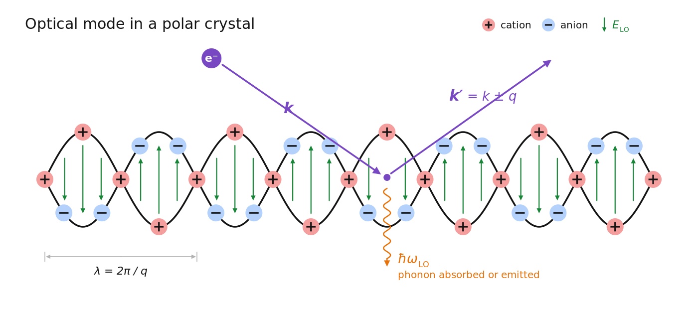
Fröhlich scattering describes the interaction of electrons and holes with longitudinal optical (LO) phonons in polar semiconductors, such as GaAs, InP, GaN, ZnO and metal-halide perovskites. The physical origin of this interaction is illustrated in ??. In a polar crystal, neighbouring atoms carry opposite partial charges. When the lattice vibrates in an optical mode, the positive and negative ions move relative to one another, producing an oscillating electric polarisation. For a longitudinal optical phonon, this generates a macroscopic electric field which interacts with charge carriers moving through the crystal.
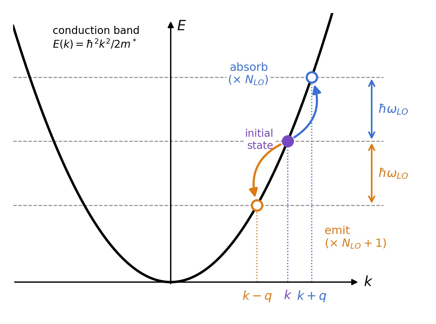
An electron travelling through this field can be scattered from an initial state with wavevector \(\mathbf{k}\) into a final state \(\mathbf{k}'\), either absorbing or emitting an LO phonon of energy \(\hbar\omega_{LO}\). These transitions are illustrated in the conduction-band diagram in ??. The electrostatic coupling between free carriers and the polarisation field of the lattice is known as the Fröhlich interaction. It is an important mechanism limiting charge carrier mobility in polar semiconductors, particularly at room temperature and above. It can dominate electron scattering in high-purity III–V materials and provides an efficient route for hot carriers to transfer energy to the lattice.
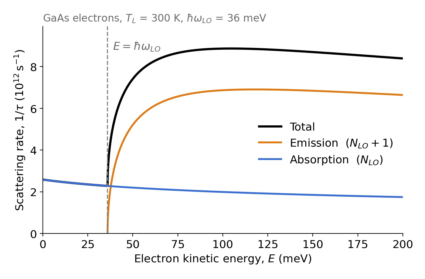
Understanding Fröhlich scattering is therefore important when calculating carrier mobility, modelling the cooling of photo-excited carriers, and determining the energy relaxation times used in energy-balance transport models. The energy dependence of the interaction can be seen in ??, which shows the calculated absorption, emission and total scattering rates for electrons in GaAs. In the following sections, we examine LO phonon absorption and emission in more detail, before deriving the Fröhlich matrix element and the full three-dimensional \(k\)-space integral used to calculate the scattering rate.
What is the Fröhlich interaction?
In a polar semiconductor, the relative displacement of positive and negative ions during a longitudinal optical (LO) vibration produces an oscillating electric field, \(\mathbf{E}_{LO}\), as illustrated in ??. A charge carrier interacts with this field through the electrostatic potential \(\phi_{LO}\), giving an interaction energy of \(-e\phi_{LO}\) for an electron. Since the interaction is Coulombic in origin, it is long-ranged and strongest at small phonon wavevectors \(q\).
The strength of the Fröhlich interaction depends on how strongly the crystal responds to an electric field. There are two contributions to this response: the electrons, which respond very quickly, and the much heavier ions, which respond more slowly. This gives rise to two dielectric constants: the high-frequency dielectric constant \(\varepsilon_\infty\), which describes the electronic response alone, and the static dielectric constant \(\varepsilon_s\), which includes the additional contribution from ionic motion.
In a polar semiconductor, the displacement of the ions during an LO phonon generates an electric field which couples to free charge carriers. The strength of this coupling is determined by the difference between the electronic and total dielectric screening, expressed as
\[ \frac{1}{\varepsilon_\infty} - \frac{1}{\varepsilon_s}. \]
The larger this quantity, the stronger the polar coupling. In a non-polar semiconductor such as silicon, there is no corresponding long-range electric field associated with optical lattice vibrations. The ionic contribution to the dielectric response is therefore absent in this model, giving \(\varepsilon_s=\varepsilon_\infty\) and a vanishing Fröhlich interaction. This dielectric term appears directly in the scattering matrix element derived below.
It is often convenient to express the coupling strength as a single dimensionless number, the Fröhlich coupling constant,
\[ \alpha = \frac{e^2}{4\pi\varepsilon_0 \hbar}\sqrt{\frac{m^*}{2\hbar\omega_{LO}}}\left(\frac{1}{\varepsilon_\infty}-\frac{1}{\varepsilon_s}\right), \]
where \(m^*\) is the carrier effective mass. For GaAs electrons \(\alpha\approx 0.07\) (weak coupling); for more ionic materials such as GaN, ZnO and the halide perovskites \(\alpha\) is of order 0.4–2. When \(\alpha\) is small, the interaction can be treated as a perturbation and gives the scattering rates derived below. When \(\alpha\) approaches or exceeds unity the carrier drags a significant polarisation cloud with it and is better described as a polaron, with a renormalised mass and energy; the perturbative rates on this page should then be used with caution.
Absorption and emission in the band picture
Fröhlich scattering is an inelastic transition in which an electron exchanges energy and momentum with an LO phonon. As illustrated in ??, an electron initially in state \(\mathbf{k}\), with energy \(E(\mathbf{k})\), can undergo one of two processes:
Phonon absorption: The electron gains energy \(\hbar\omega_{LO}\) from the lattice, moving to a higher-energy state \(\mathbf{k}'=\mathbf{k}+\mathbf{q}\), where \(E(\mathbf{k}')=E(\mathbf{k})+\hbar\omega_{LO}\).
Phonon emission: The electron transfers energy \(\hbar\omega_{LO}\) to the lattice, moving to a lower-energy state \(\mathbf{k}'=\mathbf{k}-\mathbf{q}\), where \(E(\mathbf{k}')=E(\mathbf{k})-\hbar\omega_{LO}\).
Both processes conserve energy and crystal momentum. Since LO phonons are approximately dispersionless near the zone centre, their energy \(\hbar\omega_{LO}\) can be treated as constant, approximately 36 meV in GaAs and 92 meV in GaN. This places an important restriction on emission: an electron must have at least \(\hbar\omega_{LO}\) of kinetic energy above the band minimum before it can emit an LO phonon. Electrons below this threshold can only undergo phonon absorption. Once the threshold is reached, the emission channel opens, allowing hot electrons to lose energy to the lattice in discrete amounts of \(\hbar\omega_{LO}\). This behaviour is clearly visible in ??, which shows the calculated absorption, emission and total scattering rates for electrons in GaAs.
The probability of each process also depends on the number of LO phonons present in the lattice. At thermal equilibrium, the average phonon occupation is described by the Bose–Einstein distribution,
\[ N_{LO} = \frac{1}{\exp\!\left(\hbar\omega_{LO}/k_B T_L\right)-1}, \]
where \(T_L\) is the lattice temperature. The absorption probability is proportional to \(N_{LO}\), since a phonon must already be present for the electron to absorb it. Emission, on the other hand, is proportional to \(N_{LO}+1\). The additional \(+1\) represents spontaneous phonon emission, which remains possible even at zero temperature, provided the electron has sufficient energy.
For GaAs at 300 K, \(N_{LO}\approx 0.33\), giving an emission occupation factor approximately four times larger than that for absorption. The actual scattering rates also depend on the available final electronic states, as illustrated in ??. As the lattice temperature increases, the phonon population rises, strengthening the interaction and contributing to the reduction in carrier mobility commonly observed in polar semiconductors.
The Fröhlich coupling matrix element
We now consider the interaction quantum mechanically. The coupling between an electron and a longitudinal optical phonon is described by the Fröhlich matrix element, which for a bulk polar semiconductor is given by
\[ M(q) = -\frac{i}{q} \left[ \frac{e^2\hbar\omega_{LO}}{2V\varepsilon_0} \left( \frac{1}{\varepsilon_\infty} - \frac{1}{\varepsilon_s} \right) \right]^{1/2}. \]
Here, \(V\) is the crystal normalisation volume and \(q\) is the phonon wavevector. Taking the electronic states to be plane waves, the interaction connects an initial state \(|\mathbf{k}\rangle\) to a final state \(|\mathbf{k}'\rangle\), subject to conservation of crystal momentum. For phonon absorption and emission, respectively, the final wavevector is \(\mathbf{k}'=\mathbf{k}\pm\mathbf{q}\).
Including the phonon occupation factors, and assuming the overlap between the periodic parts of the initial and final Bloch functions is approximately unity, the squared transition matrix elements become
\[ |M_{\mathrm{abs}}(q)|^2 = |M(q)|^2 N_{LO}, \]
\[ |M_{\mathrm{em}}(q)|^2 = |M(q)|^2 (N_{LO}+1). \]
The absorption term depends on the number of available LO phonons, while emission contains an additional spontaneous contribution. These matrix elements are used in Fermi's golden rule to calculate the probability of a transition between electronic states.
From Fermi's golden rule to a 3D k-space integral
Having established the Fröhlich coupling matrix element, we can now calculate the rate at which an electron scatters from an initial state \(|\mathbf{k}\rangle\) into a final state \(|\mathbf{k}'\rangle\). As illustrated in ??, this can occur through either LO phonon absorption or emission, with the electron gaining or losing an energy \(\hbar\omega_{LO}\).
Using Fermi's golden rule, the total out-scattering rate is obtained by summing over all allowed phonon wavevectors \(\mathbf{q}\) and both scattering processes:
\[ \begin{aligned} \frac{1}{\tau(\mathbf{k})} = \frac{2\pi}{\hbar} \sum_{\mathbf{q}} \Big[ &|M_{\mathrm{abs}}(q)|^2 \delta\big( E(\mathbf{k}+\mathbf{q})-E(\mathbf{k})-\hbar\omega_{LO} \big) \\ +{}& |M_{\mathrm{em}}(q)|^2 \delta\big( E(\mathbf{k}-\mathbf{q})-E(\mathbf{k})+\hbar\omega_{LO} \big) \Big]. \end{aligned} \]
Here, \(\delta\) is the Dirac delta function, which enforces conservation of energy. The absorption and emission matrix elements, \(|M_{\mathrm{abs}}(q)|^2=|M(q)|^2N_{LO}\) and \(|M_{\mathrm{em}}(q)|^2=|M(q)|^2(N_{LO}+1)\), were introduced in the previous section. We assume that the final electronic states are unoccupied, so that Pauli blocking can be neglected.
For a sufficiently large crystal, the allowed phonon wavevectors are closely spaced and the sum can be replaced by an integral over the Brillouin zone:
\[ \sum_{\mathbf{q}} \longrightarrow \frac{V}{(2\pi)^3}\int d^3q. \]
The factor of \(V\) cancels the \(1/V\) dependence of the squared Fröhlich matrix element, leaving a scattering rate that is independent of the crystal normalisation volume. Substituting the expression for \(M_{\mathrm{abs}}(q)\), the absorption rate becomes
\[ \begin{aligned} \frac{1}{\tau_{\mathrm{abs}}(\mathbf{k})} ={}& \frac{2\pi}{\hbar} \frac{V}{(2\pi)^3} \int d^3q\; \frac{e^2\hbar\omega_{LO}}{2V\varepsilon_0} \left( \frac{1}{\varepsilon_\infty} - \frac{1}{\varepsilon_s} \right) \frac{N_{LO}}{q^2} \\[4pt] &\times \delta\big( E(\mathbf{k}+\mathbf{q})-E(\mathbf{k})-\hbar\omega_{LO} \big). \end{aligned} \]
To evaluate this integral, we use spherical coordinates with the polar axis aligned along the initial electron wavevector \(\mathbf{k}\). Integrating over the azimuthal angle gives
\[ d^3q = 2\pi q^2\,dq\,d(\cos\theta), \]
where \(\theta\) is the angle between the electron and phonon wavevectors, \(\mathbf{k}\) and \(\mathbf{q}\). Notice that the \(q^2\) contribution from the volume element cancels the \(1/q^2\) dependence of the Fröhlich matrix element. This simplifies the remaining integration considerably.
Assuming a parabolic, isotropic conduction band, \(E(\mathbf{k})=\hbar^2k^2/2m^*\), the argument of the absorption delta function can be expanded as
\[ \begin{aligned} &E(\mathbf{k}+\mathbf{q})-E(\mathbf{k})-\hbar\omega_{LO} \\[4pt] &\qquad = \frac{\hbar^2}{2m^*} \left( 2kq\cos\theta+q^2 \right) -\hbar\omega_{LO}. \end{aligned} \]
Integration over \(\cos\theta\) removes the delta function and contributes a factor \(m^*/(\hbar^2kq)\), provided the solution satisfies \(-1\leq\cos\theta\leq1\). This condition restricts the range of allowed phonon wavevectors according to conservation of energy and crystal momentum.
For phonon absorption, the allowed limits are
\[ \begin{aligned} q_{\min} &= k'-k,\\ q_{\max} &= k'+k,\\ k' &= \sqrt{k^2+\frac{2m^*\omega_{LO}}{\hbar}}. \end{aligned} \]
For phonon emission, which requires \(E\geq\hbar\omega_{LO}\), the corresponding limits are
\[ \begin{aligned} q_{\min} &= k-k',\\ q_{\max} &= k+k',\\ k' &= \sqrt{k^2-\frac{2m^*\omega_{LO}}{\hbar}}. \end{aligned} \]
The remaining radial integration is straightforward:
\[ \int_{q_{\min}}^{q_{\max}} \frac{dq}{q} = \ln\left(\frac{q_{\max}}{q_{\min}}\right). \]
Collecting the terms and using \(\hbar k=\sqrt{2m^*E}\), where \(E\) is the carrier kinetic energy measured relative to the band minimum, gives the standard closed-form expressions for the Fröhlich scattering rates. For absorption,
\[ \boxed{ \begin{aligned} \frac{1}{\tau_{\mathrm{abs}}(E)} ={}& C(E)N_{LO} \\ &\times \ln\left| \frac{ \sqrt{E+\hbar\omega_{LO}}+\sqrt{E} }{ \sqrt{E+\hbar\omega_{LO}}-\sqrt{E} } \right|, \end{aligned} } \]
while for emission,
\[ \boxed{ \begin{aligned} \frac{1}{\tau_{\mathrm{em}}(E)} ={}& C(E)(N_{LO}+1) \\ &\times \ln\left| \frac{ \sqrt{E}+\sqrt{E-\hbar\omega_{LO}} }{ \sqrt{E}-\sqrt{E-\hbar\omega_{LO}} } \right|, \qquad E\geq\hbar\omega_{LO}. \end{aligned} } \]
The emission rate is zero below the LO phonon energy threshold. In these expressions, the common prefactor is
\[ C(E)= \frac{e^2\omega_{LO}}{4\pi\varepsilon_0\hbar} \left( \frac{1}{\varepsilon_\infty} - \frac{1}{\varepsilon_s} \right) \sqrt{\frac{m^*}{2E}}. \]
The total Fröhlich out-scattering rate is simply the sum of the two contributions:
\[ \boxed{ \frac{1}{\tau(E)} = \frac{1}{\tau_{\mathrm{abs}}(E)} + \frac{1}{\tau_{\mathrm{em}}(E)}. } \]
The common prefactor can also be expressed using the dimensionless Fröhlich coupling constant \(\alpha\), giving \(C(E)=\alpha\omega_{LO}\sqrt{\hbar\omega_{LO}/E}\). Two limits are worth noting. As \(E\rightarrow0\), the absorption rate approaches the finite value \(2\alpha\omega_{LO}N_{LO}\). At the emission threshold, \(E=\hbar\omega_{LO}\), the emission contribution begins at zero and rises rapidly with increasing carrier energy.
This behaviour can be seen directly in ??, which shows the calculated absorption, emission and total scattering rates for electrons in GaAs at 300 K. For hot electrons, the resulting rates are typically of order \(10^{12}\)–\(10^{13}\,\mathrm{s^{-1}}\), with LO phonon emission times reaching approximately 0.1–0.2 ps. These rapid emission processes provide an important mechanism through which energetic carriers transfer energy to the lattice.
From carrier scattering to mobility
Charge carrier scattering plays an important role in determining the electrical mobility of a semiconductor. When an electric field is applied, electrons and holes accelerate under the force of the field. However, their motion is continually interrupted by interactions with phonons, impurities, defects and other carriers. These scattering processes prevent carriers from accelerating indefinitely and determine their average drift velocity.
In the simplest transport model, the relationship between carrier mobility and scattering is described by the Drude expression,
\[ \boxed{ \mu = \frac{e\tau_{\mathrm{tr}}}{m^*} } \]
where \(e\) is the elementary charge, \(m^*\) is the carrier effective mass, and \(\tau_{\mathrm{tr}}\) is the momentum relaxation time. Physically, \(\tau_{\mathrm{tr}}\) describes how quickly scattering removes the directed motion of carriers produced by an applied electric field. A longer relaxation time generally leads to a higher mobility, whereas stronger momentum relaxation reduces it.
From scattering rate to momentum relaxation
There is an important distinction between the total scattering rate calculated in the previous section and the rate at which scattering relaxes carrier momentum. The total out-scattering rate, \(1/\tau(\mathbf{k})\), counts every transition out of an initial electronic state, irrespective of how much the direction of carrier motion changes.
Consider an electron travelling with an initial wavevector \(\mathbf{k}\). Following a scattering event, its wavevector changes to \(\mathbf{k}'\), making an angle \(\theta_s\) with its original direction. For an isotropic parabolic band and an elastic scattering event, the electron retains the same speed, but only a component of its final velocity remains parallel to its original direction. This component is
\[ v_{\parallel}' = v\cos\theta_s. \]
The fraction of the original directed velocity lost during the scattering event is therefore
\[ \frac{v-v_{\parallel}'}{v} = \boxed{1-\cos\theta_s}. \]
This simple geometric argument explains why scattering through different angles does not contribute equally to momentum relaxation. For example:
- Forward scattering (\(\theta_s=0^\circ\)): the weighting is zero, since the electron continues in its original direction.
- Scattering through \(90^\circ\): the weighting is one, since none of the original directed velocity remains.
- Backscattering (\(\theta_s=180^\circ\)): the weighting is two, since the electron reverses its direction of motion.
We can use this angular dependence to construct an approximate transport scattering rate. For isotropic bands, a commonly used angular-weighting approximation is
\[ \begin{aligned} \frac{1}{\tau_{\mathrm{tr}}(\mathbf{k})} \simeq \frac{2\pi}{\hbar} \sum_{\mathbf{q}} (1-\cos\theta_s) \Big[ &|M_{\mathrm{abs}}(q)|^2 \delta(E'-E-\hbar\omega_{LO}) \\ +{}& |M_{\mathrm{em}}(q)|^2 \delta(E'-E+\hbar\omega_{LO}) \Big]. \end{aligned} \]
Here, \(\theta_s\) is the angle between the initial and final carrier velocities. For an isotropic parabolic band, these velocities are parallel to their corresponding wavevectors. The matrix elements \(M_{\mathrm{abs}}\) and \(M_{\mathrm{em}}\) are those derived in the previous section.
For inelastic scattering, where the carrier speed also changes, the simple angular weighting is an approximation. A more general single-event projection factor is \(1-(v'/v)\cos\theta_s\) for an isotropic band. A rigorous treatment of inelastic transport requires solving the linearised Boltzmann transport equation, which accounts for the coupling between initial and final carrier states.
This distinction is particularly relevant to Fröhlich scattering. Since the interaction favours small phonon wavevectors \(q\), many transitions involve relatively small changes in the carrier direction. The total scattering rate can therefore be considerably different from the rate at which directed carrier motion is relaxed.
Calculating mobility from the band structure
The Drude expression provides a useful starting point, but real semiconductors do not necessarily have a single effective mass or a constant relaxation time. Both the scattering rate and the carrier velocity can vary across the electronic band structure.
To account for this, mobility can be calculated by averaging the contributions from the electronic states involved in transport. Within the relaxation-time approximation, the electron mobility tensor is
\[ \boxed{ \mu_{ij} = \frac{e}{n} \sum_b \int \frac{d^3k}{(2\pi)^3} v_{b,i}(\mathbf{k}) v_{b,j}(\mathbf{k}) \tau_{\mathrm{tr},b}(\mathbf{k}) \left( -\frac{\partial f}{\partial E} \right)_{E_b(\mathbf{k})} } \]
Here, \(n\) is the electron density, \(f\) is the Fermi–Dirac distribution, and the sum runs over the relevant electronic bands and explicitly represented spin or valley states. The group velocity of each state is obtained from the band dispersion,
\[ \mathbf{v}_b(\mathbf{k}) = \frac{1}{\hbar} \nabla_{\mathbf{k}}E_b(\mathbf{k}). \]
The derivative of the Fermi–Dirac distribution determines which electronic states contribute to the electrical response. The integral then combines their velocities and transport relaxation times to obtain the overall mobility.
This approach is particularly useful for numerical band structures, such as those calculated using \(k\cdot p\) theory, since the energy-dependent velocities can be obtained directly from the calculated dispersion rather than assuming a constant effective mass. It also allows different scattering mechanisms to be included through their contributions to the transport relaxation time.