

AlGaAs/GaAs Heterojunction Diode Simulation: Band Alignment, J–V Curves and Carrier Transport
1. Introduction: why simulate an AlGaAs/GaAs heterojunction?
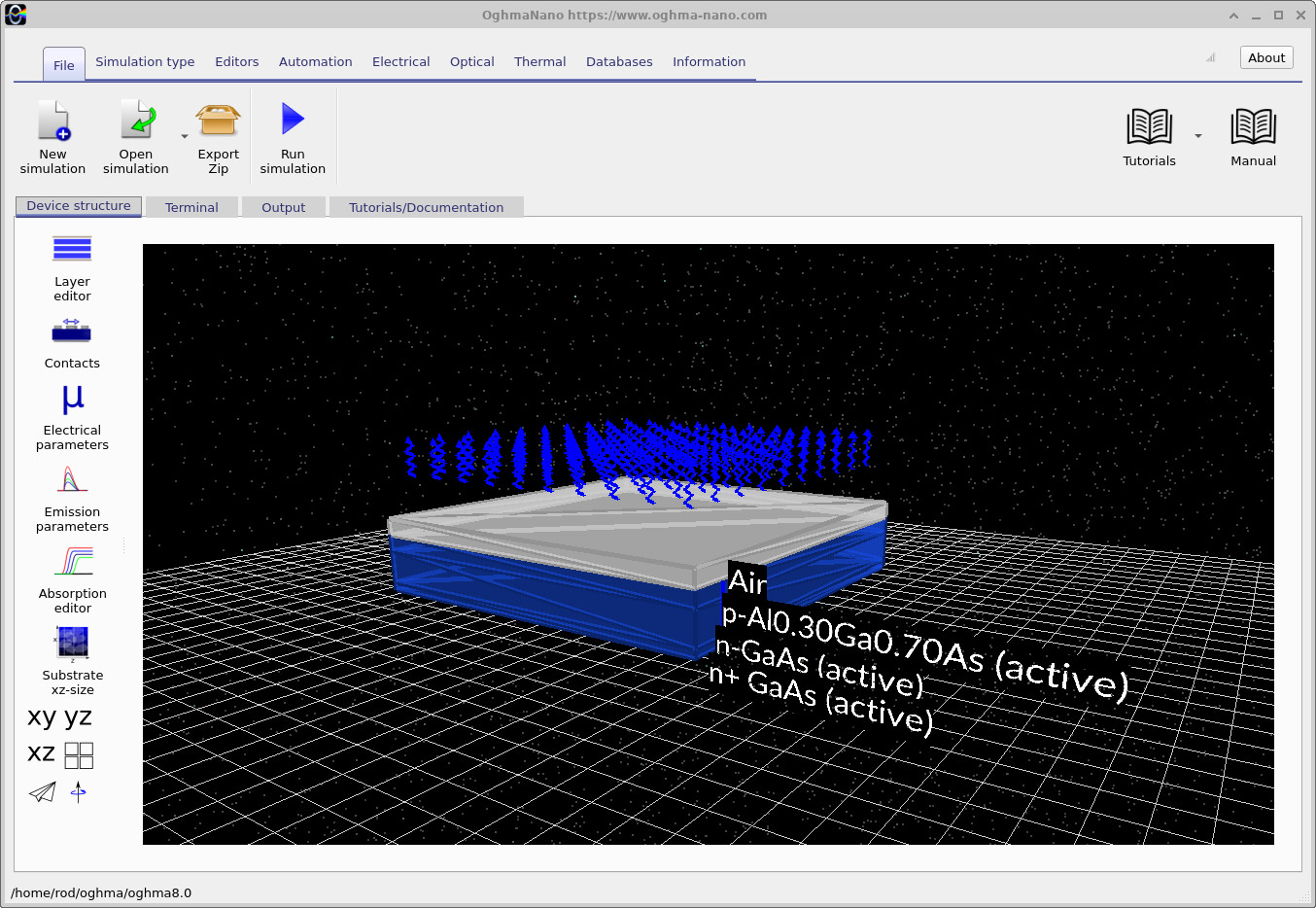
An AlGaAs/GaAs heterojunction diode is a semiconductor diode formed where two different III–V materials meet: aluminium gallium arsenide (AlxGa1−xAs) and gallium arsenide (GaAs). Unlike a conventional GaAs PN diode, this device combines a change in doping with a change in semiconductor band structure. The junction therefore exhibits both a built-in electrostatic potential and offsets between the conduction and valence bands.
In this tutorial we study a p-Al0.30Ga0.70As / n-GaAs junction using OghmaNano's one-dimensional Poisson and drift–diffusion solver. The wider-bandgap AlGaAs region meets the narrower-bandgap GaAs region; their interface modifies electron and hole injection and provides a simple introduction to heterojunction band alignment. The complete semiconductor stack is only 700 nm thick, making it convenient for visualising internal transport profiles.
AlGaAs/GaAs heterostructures are important building blocks in III–V electronics and optoelectronics, including heterojunction devices, photovoltaic window layers and light-emitting structures. This example is specifically a diode/rectifier demonstration: it is not presented as an optimised photodiode, laser diode or commercial high-speed component. We will use the model to connect a measurable dark current-density–voltage (J–V) characteristic with the microscopic band diagram and recombination physics.
The main view is shown in ?? . The remainder of the tutorial follows the same progression as the other OghmaNano diode examples: load a device, inspect its inputs, run a simulation, and interpret the results.
2. Making a new simulation
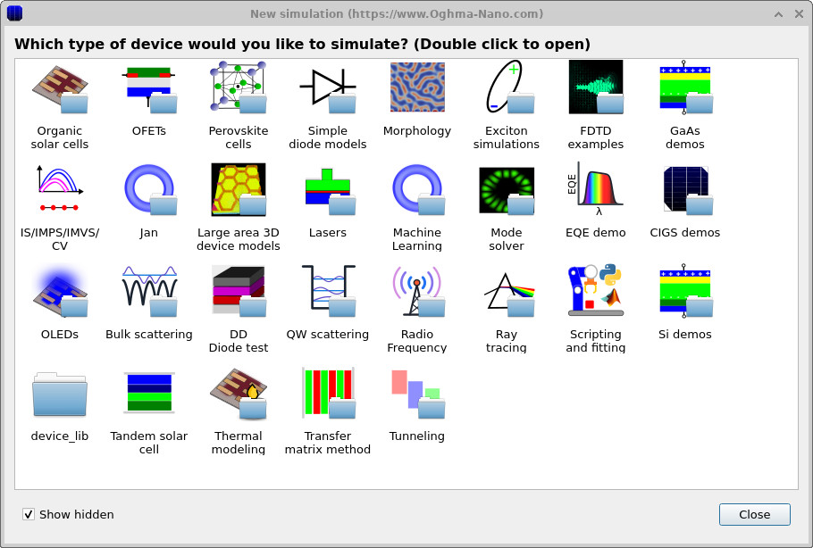
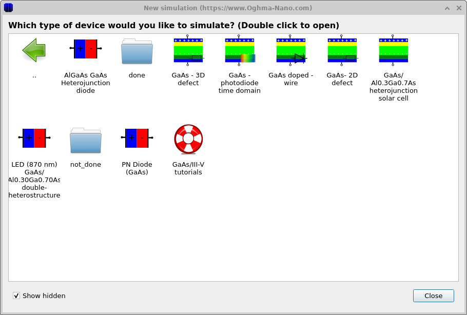
From the OghmaNano main window, select New simulation. The demonstration browser groups related semiconductor examples. Open the GaAs/III–V demonstrations and select the AlGaAs/GaAs heterojunction diode example, or load the supplied example project directly if its menu label differs between versions. The two stages of the browser are shown in ?? and ?? .
Once the example opens, inspect the vertical stack in the device view. Although the viewer is three-dimensional, this tutorial solves one-dimensional electrical transport through the layer thickness. The model does not resolve lateral current crowding or real metal-contact geometries.
3. Examining the layer structure, alloy composition and doping
3.1 Layer stack
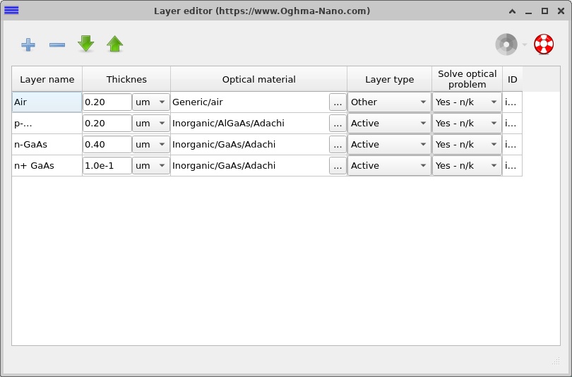
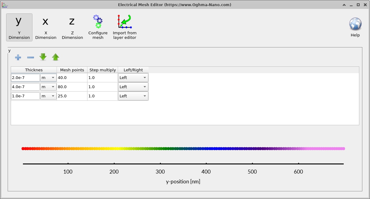
Open the Layer editor from the device ribbon. The active diode comprises three semiconductor layers, with an air region above them for the device representation. The electrical problem spans the 700 nm semiconductor stack rather than the 200 nm air region.
| Region (top to bottom) | Thickness | Doping in the model | Purpose |
|---|---|---|---|
| Air (not electrically active) | 200 nm | — | Environment above the device |
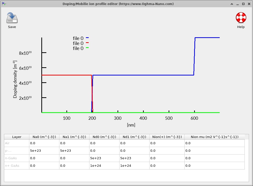
| p-Al0.30Ga0.70As | 200 nm | NA = 5 × 1017 cm−3 | Wide-bandgap p-side of heterojunction |
| n-GaAs | 400 nm | ND = 5 × 1017 cm−3 | Narrower-bandgap n-side |
| n+-GaAs | 100 nm | ND = 1 × 1018 cm−3 | Heavier-doped cathode-side region |
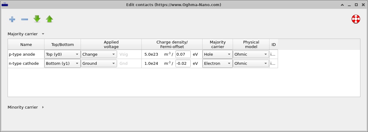
The p-AlGaAs/n-GaAs boundary is both the metallurgical PN junction and the material interface. The n-GaAs/n+-GaAs boundary is a doping transition within GaAs, not a second heterojunction. The layer editor (??) and contact configuration (??) are shown together below.
3.2 Doping and aluminium composition
Open the Doping / Ions editor from the Electrical ribbon. The acceptor-doped AlGaAs side and donor-doped GaAs side form the rectifying junction (??). The doping changes sign at the material interface, establishing a built-in electric field. The n+ region raises the electron concentration near the cathode.
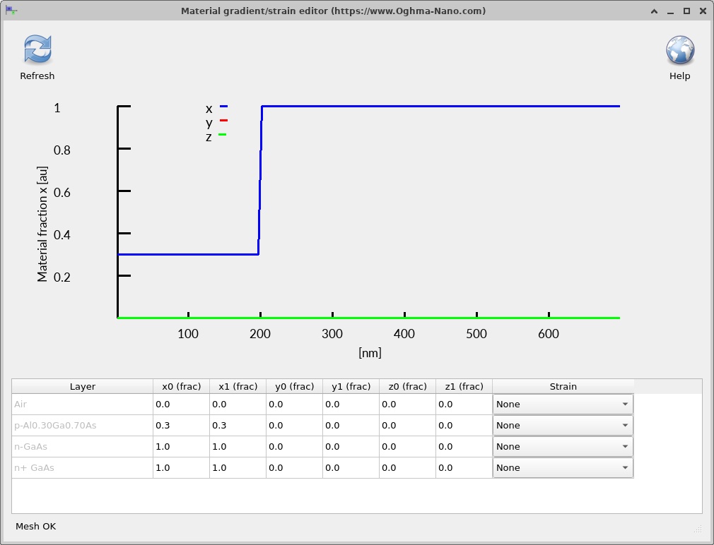
Next open the alloy composition/gradients editor. The AlGaAs alloy has an aluminium mole fraction of x = 0.30, while GaAs corresponds to x = 0. The abrupt composition step (??) is a key reason the band-edge diagram contains a step in addition to ordinary electrostatic band bending.
3.3 Why the interface matters
At room temperature GaAs has a bandgap near 1.42 eV, while Al0.30Ga0.70As has a larger bandgap, often around 1.8 eV depending on the alloy parameterisation. In a heterojunction the total bandgap difference is distributed between conduction- and valence-band offsets:
\[\Delta E_g = \Delta E_c + \Delta E_v\]Here the offset symbols denote the magnitudes of the corresponding steps. Their numerical values are determined by the material model and band-alignment assumptions, not by the doping profile alone. When examining the simulated band edges later, distinguish a sharp material-related offset from the smooth band bending produced by space charge.
4. Electrical material parameters, interfaces and recombination
4.1 The material database and Lua models
Open the Electrical parameters editor for each layer. This example uses Inorganic/AlGaAs/AlGaAs.lua for the p-type alloy and Inorganic/GaAs/GaAs.lua for both n-type GaAs regions. The AlGaAs Lua model (??) and its parameters (??) can be compared with the GaAs model (??) and its parameters (??).
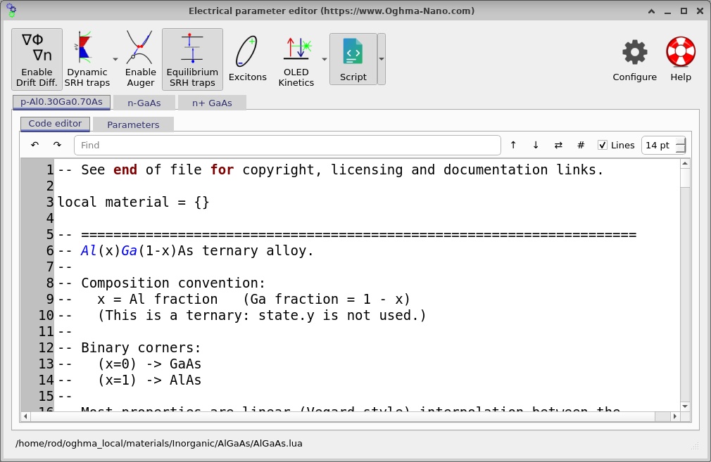
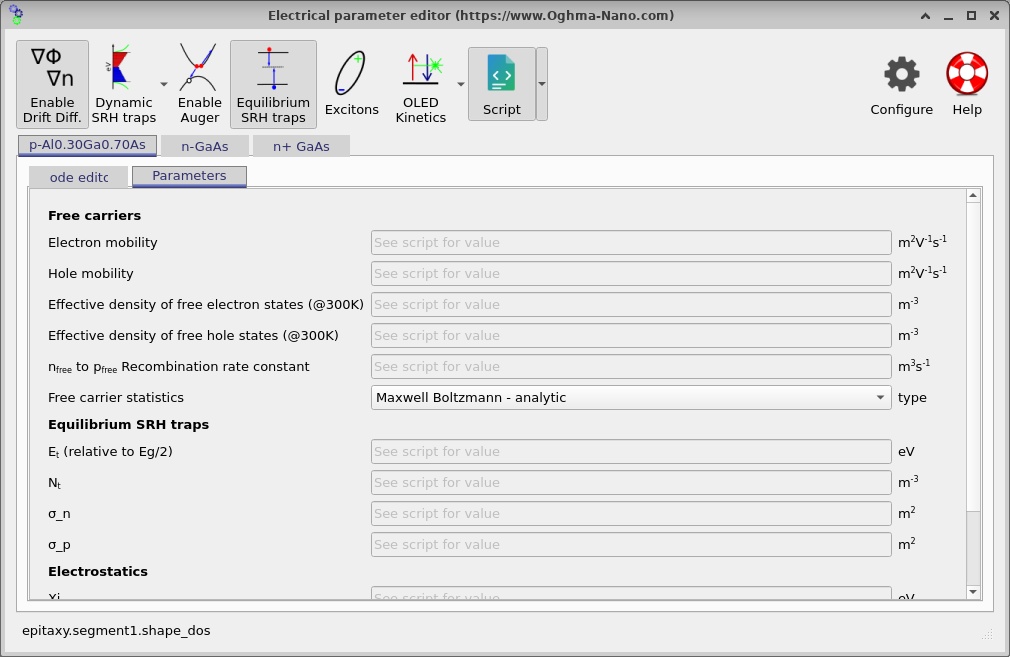
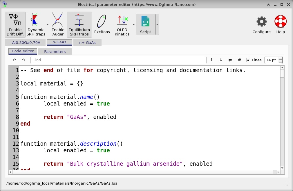
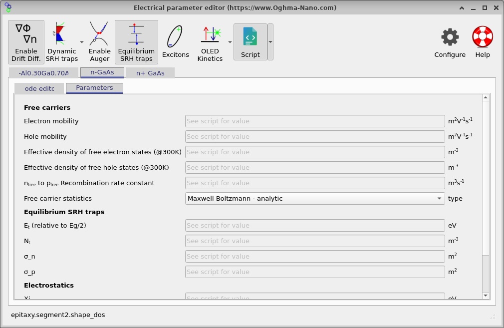
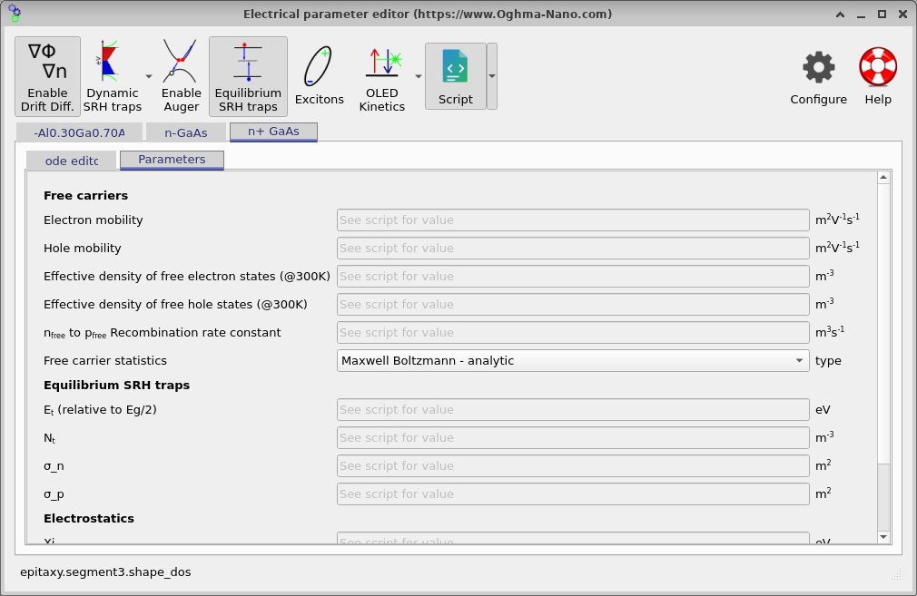
The simulation is configured to take key material values—including the bandgap, electron affinity, carrier mobilities, effective densities of states and recombination parameters—from the Lua material database rather than forcing local overrides. This is particularly important for AlGaAs because its parameters depend on the alloy composition. Read the on-screen values returned by the model, rather than interpreting any inactive fallback numbers in the project file as the material's actual properties.
4.2 Band alignment and interface settings
Open the Interfaces editor, shown in ?? . This example represents an abrupt interface. In a basic drift–diffusion treatment, carrier injection depends on the conduction- and valence-band discontinuities, carrier statistics and the interface boundary treatment. Real samples may additionally exhibit interface states, alloy disorder, thermionic emission, tunnelling or processing-induced imperfections; those effects should not be assumed to be included simply because a heterojunction is present.
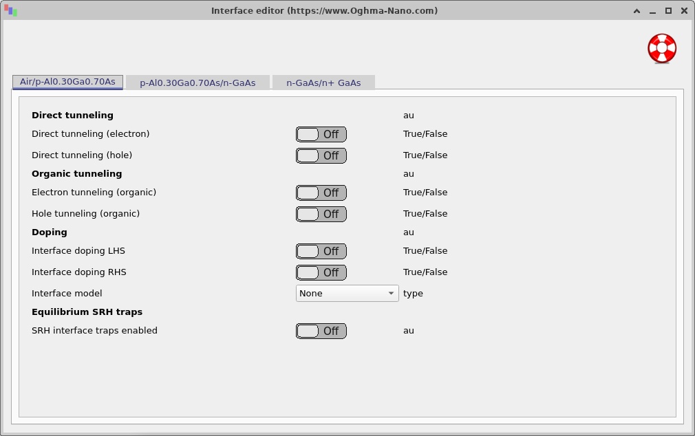
4.3 Radiative and defect-assisted recombination
GaAs and Al0.30Ga0.70As are direct-gap materials at this composition, so free-to-free radiative recombination can contribute under carrier injection. A common model is:
\[R_{\mathrm{rad}} = B\left(np-n_i^2\right)\]where B is a material-dependent coefficient and n and p are the local free-carrier densities. The input configuration also enables single-level Shockley–Read–Hall (SRH) recombination in the three active semiconductor regions. An idealised expression is:
\[R_{\mathrm{SRH}}=\frac{np-n_i^2}{\tau_p(n+n_1)+\tau_n(p+p_1)}\]SRH describes trap-assisted recombination and is sensitive to the trap parameters provided by the chosen models. Auger recombination is disabled in this example. You should not conclude that one recombination process dominates without comparing its magnitude with the other enabled processes under the same bias conditions.
The anode and cathode use idealised ohmic boundary conditions. These help isolate the heterojunction physics but do not predict the behaviour of a particular metallisation scheme or its contact resistance.
5. Running the dark J–V simulation
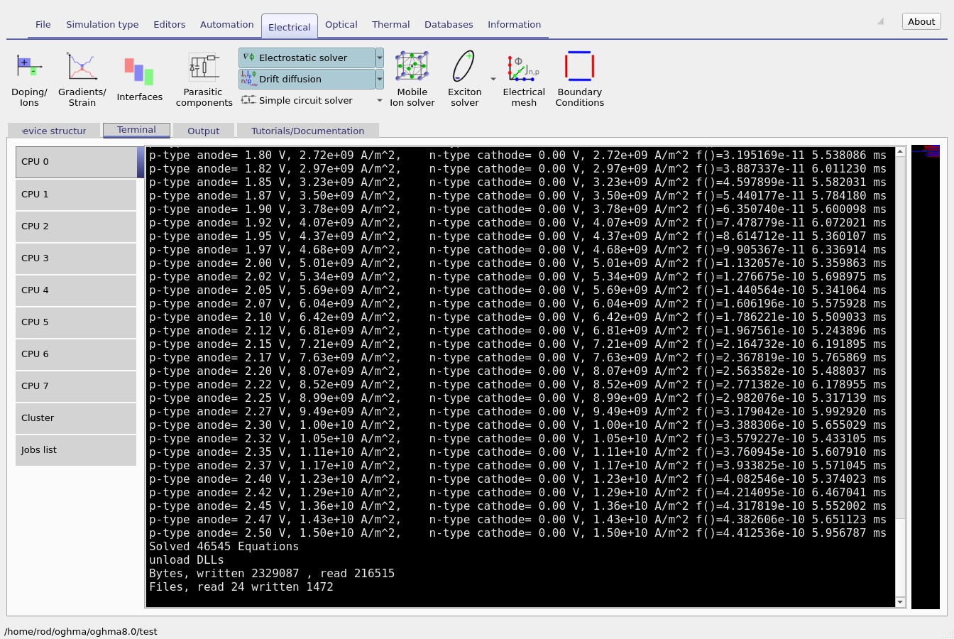
Return to the main simulation window and click Run simulation. The input file specifies a voltage sweep from −0.1 V to +2.5 V in increments of 0.025 V, without deliberate optical illumination. OghmaNano solves the coupled Poisson and electron/hole continuity equations at successive bias points.
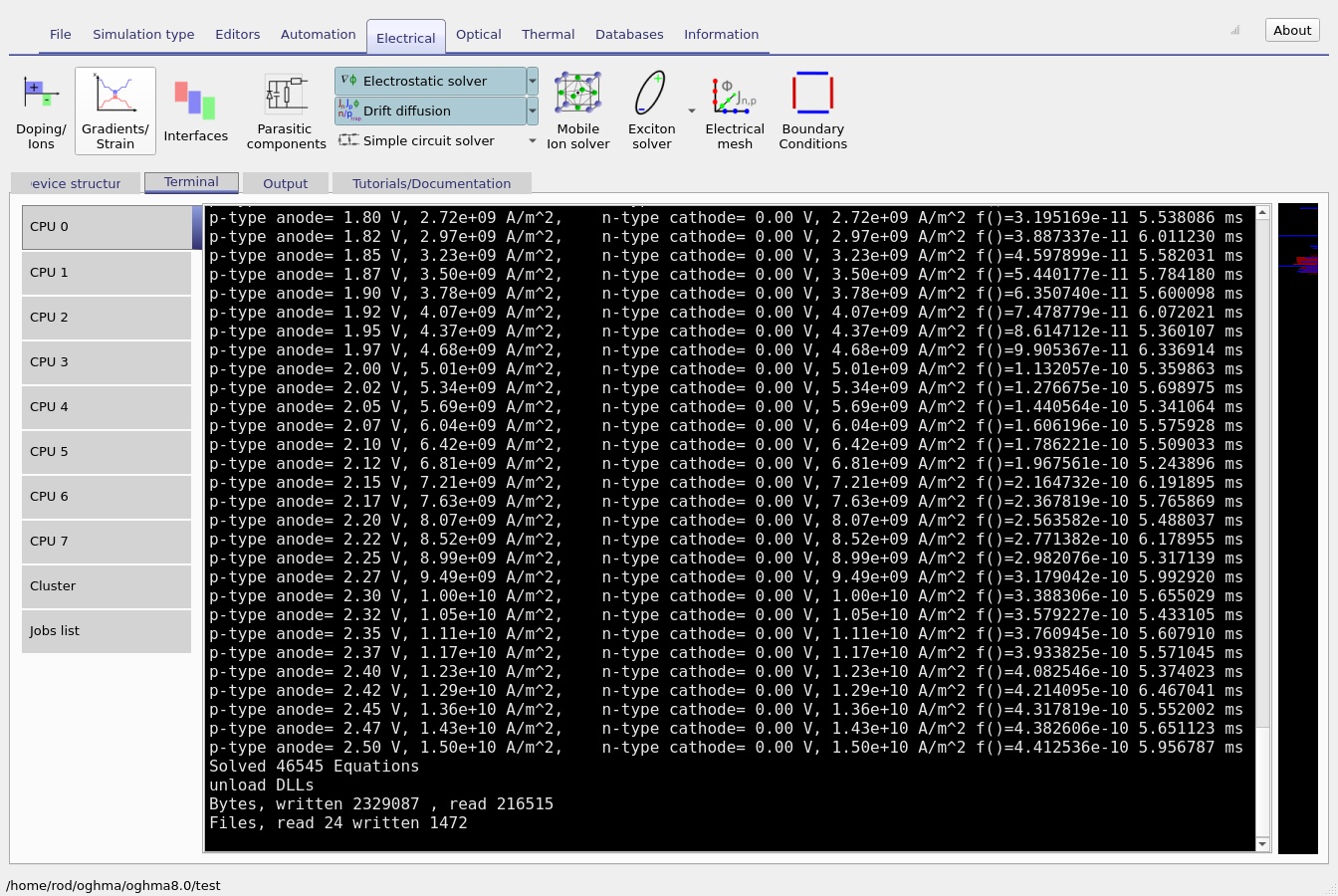
During the calculation, switch to the Terminal tab to watch solver progress, then open Output after completion. The output browser (??) and terminal (??) illustrate these stages. The terminal screenshots are captured at different elapsed times, not at fixed electrical biases.
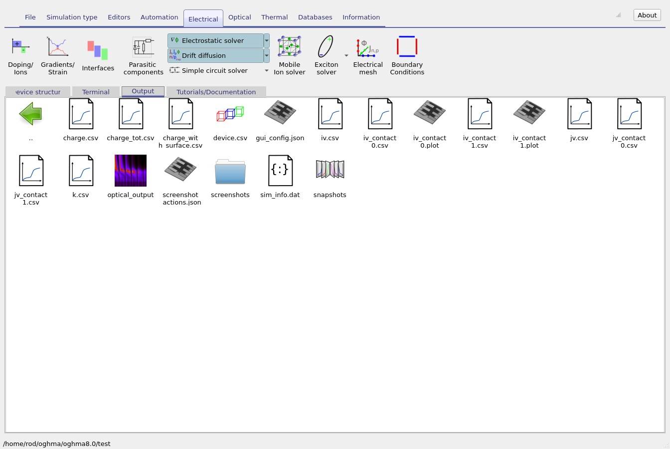
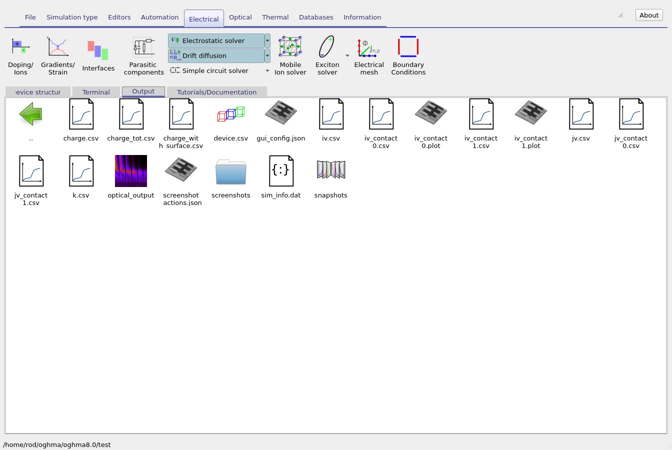
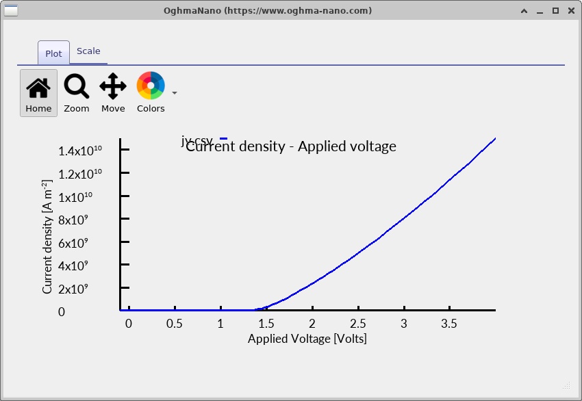
Double-click jv.csv to open the simulated current-density–voltage curve (
??
). A rectifying characteristic should exhibit relatively weak current under modest reverse bias and an increasingly large forward current as injection increases. For this particular heterojunction, the onset and detailed shape depend on the band offsets, material parameters and recombination rates—not just the GaAs bandgap.
The ideal-diode expression can be useful as a local interpretation tool:
\[J \approx J_0\left[\exp\!\left(\frac{qV}{nk_{\mathrm B}T}\right)-1\right]\]However, a fitted ideality factor n or saturation current J0 should only be extracted from a suitable voltage interval. Series resistance, high injection and heterointerface transport may cause departures from a simple exponential law. The supplied screenshot is illustrative, not an independent experimental validation.
6. Examining simulation snapshots: what happens inside the diode?
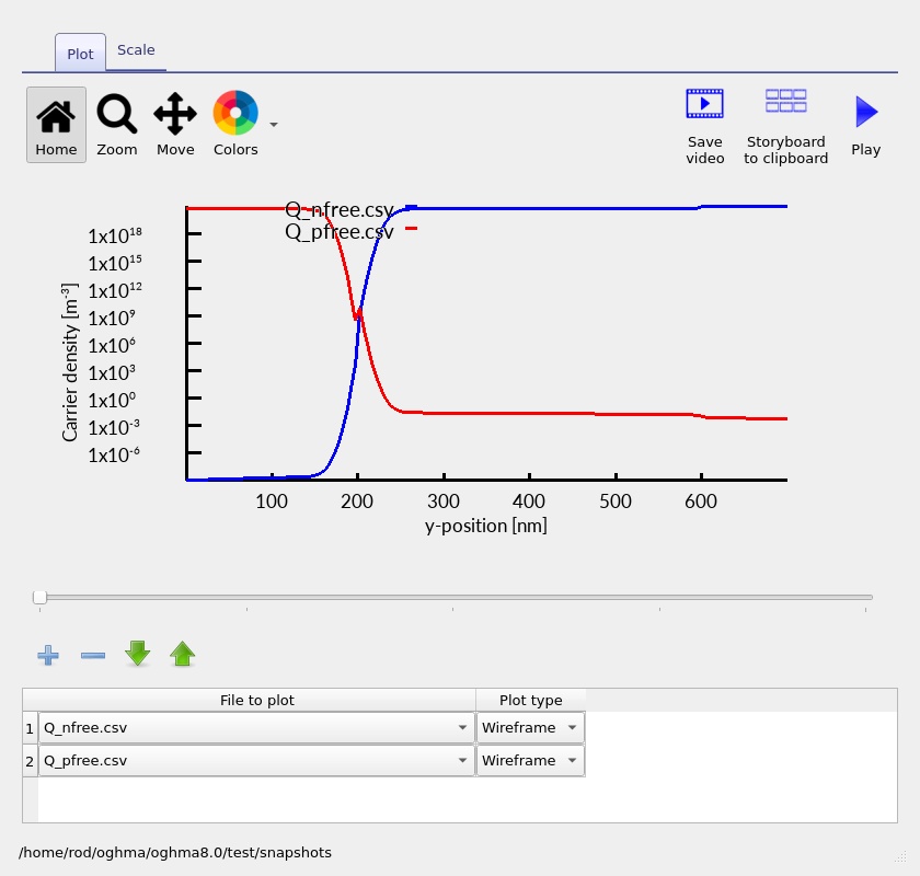
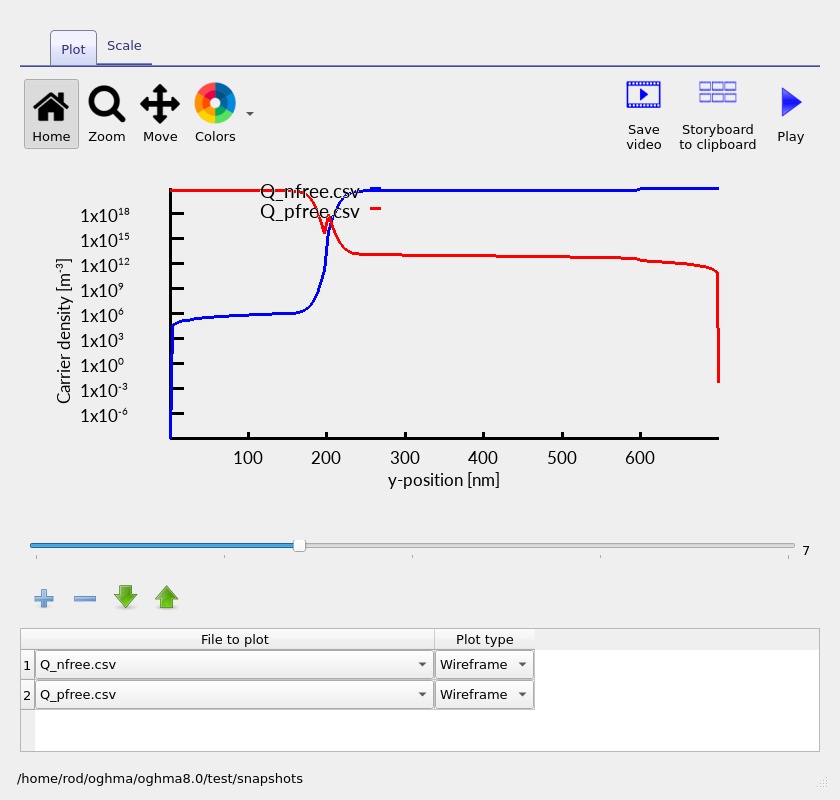
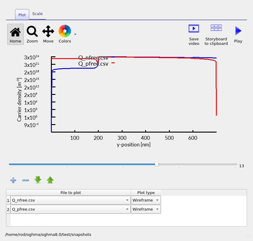
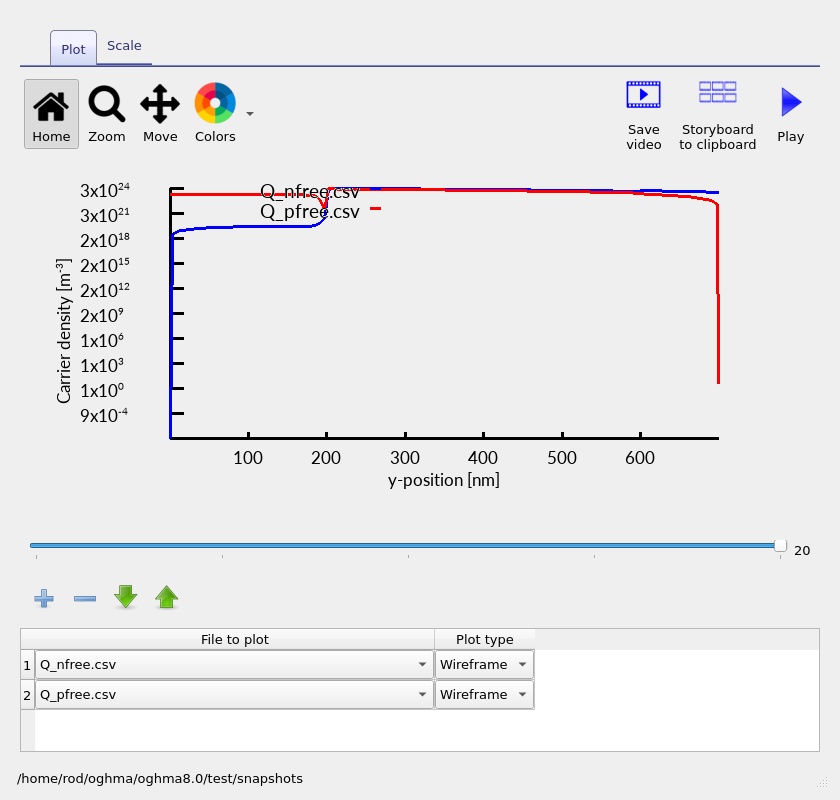
OghmaNano saves spatially resolved electrical results during the J–V sweep. Open the snapshots viewer and use its slider to compare selected bias positions. The four images in each row below correspond to the start, approximately one-third, approximately two-thirds and end of the saved sweep. The labels 0–3 indicate screenshot positions, not voltages in volts; use the viewer's bias readout to obtain the exact values for a particular run.
6.1 Conduction band, valence band and quasi-Fermi levels
Plot Ec.csv, Ev.csv, Fn.csv and Fp.csv together. The first band-diagram screenshot (??) shows the conduction-band edge Ec and valence-band edge Ev show both the smooth electrostatic potential and the abrupt band discontinuity at the AlGaAs/GaAs material interface. The electron and hole quasi-Fermi levels reveal departures from equilibrium and the distribution of injected carriers.
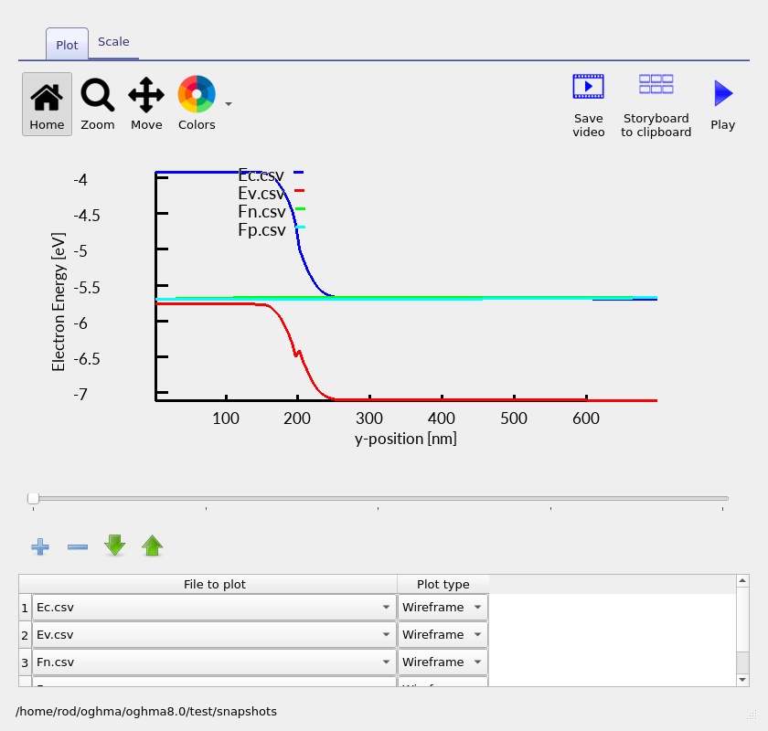
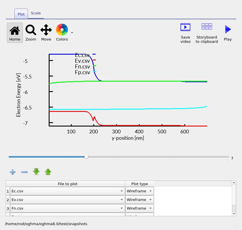
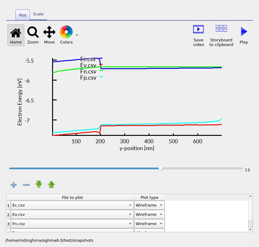
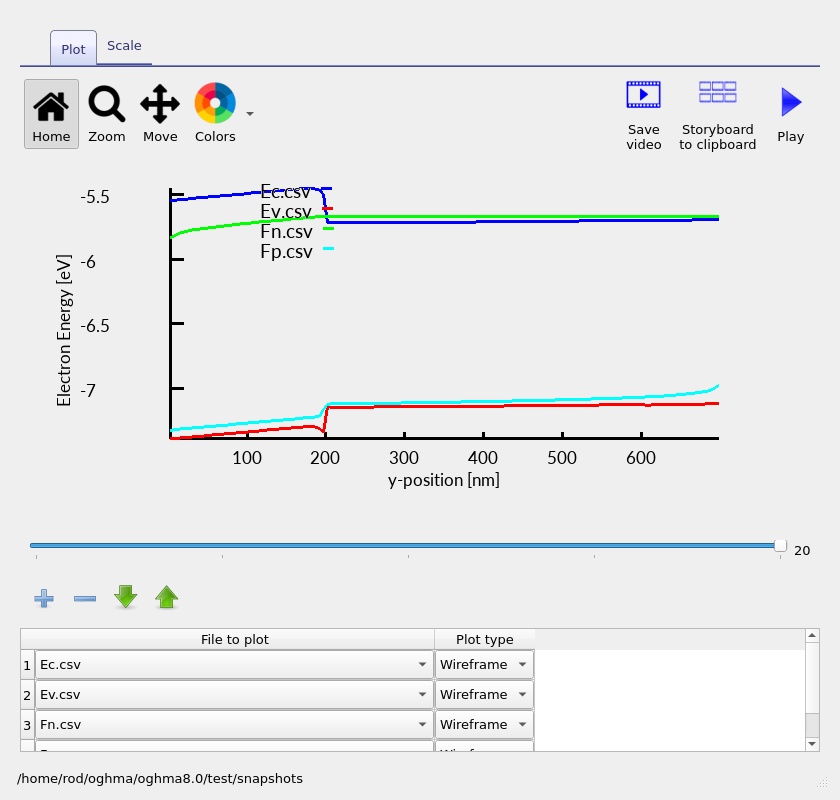
Compare the first and last images. Under forward bias the junction barrier changes and the quasi-Fermi levels separate. Do not mistake a band-edge step at the interface for numerical noise: a genuine heterojunction can have discontinuous band edges even while the electrostatic potential remains continuous.
6.2 Electron and hole densities
Plot the free-electron and free-hole population outputs, Q_nfree.csv and Q_pfree.csv in this project. The p-AlGaAs side is majority-hole material and the GaAs side is majority-electron material. Increasing forward bias injects minority carriers across the junction and changes the spatial carrier distributions. As the carrier-density results (??) illustrate, an abrupt material boundary changes the available electronic states and band alignment, so the carrier-density profile need not resemble that of a homogeneous GaAs PN junction.
6.3 Electron and hole currents
Plot Jn.csv and Jp.csv to separate the electron and hole contributions to the total current. In steady state, the two components can redistribute with position as electrons and holes recombine, while the sum of the signed electrical current densities should remain approximately conserved in the absence of additional current sources. Local peaks or rapid changes near the heterojunction in the carrier-current plots (??) should be checked against the mesh and band diagram.
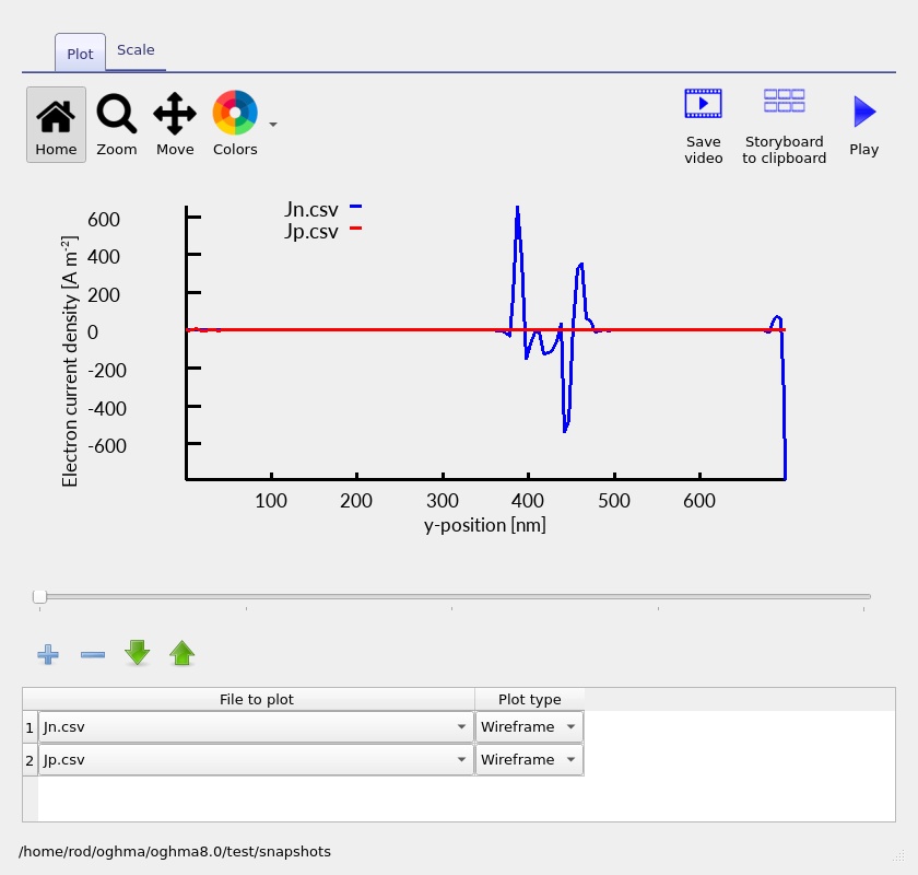
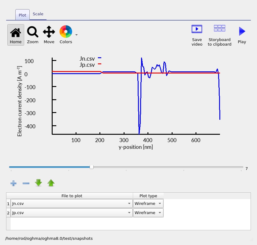
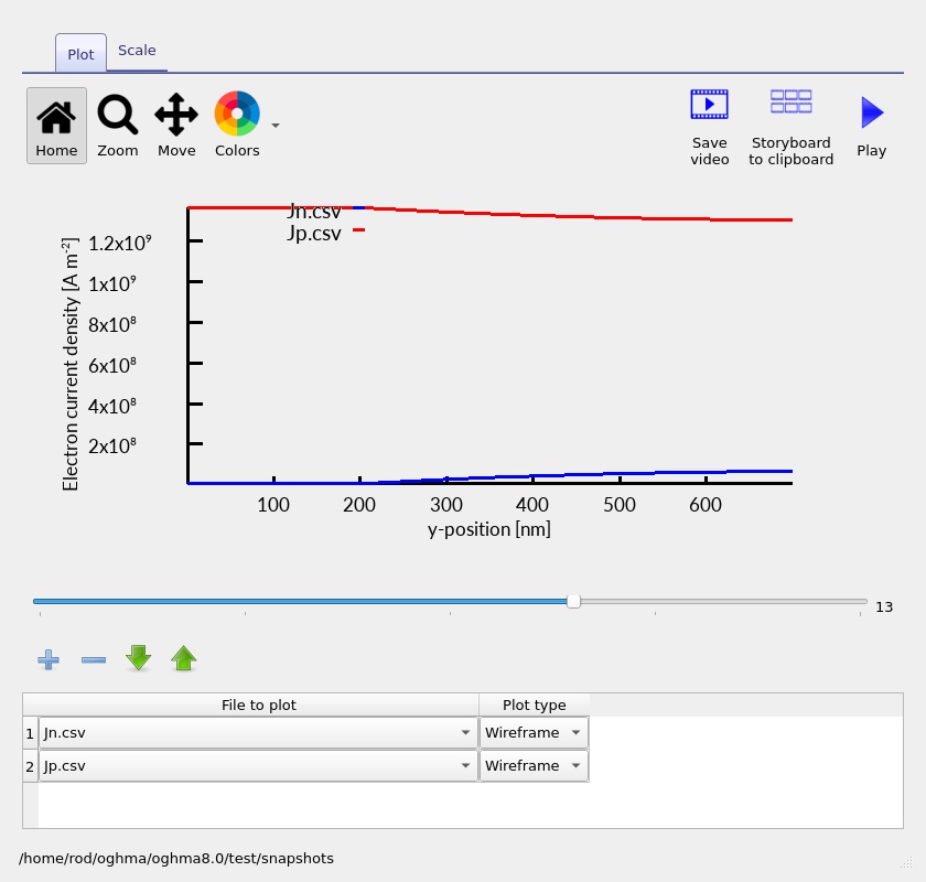
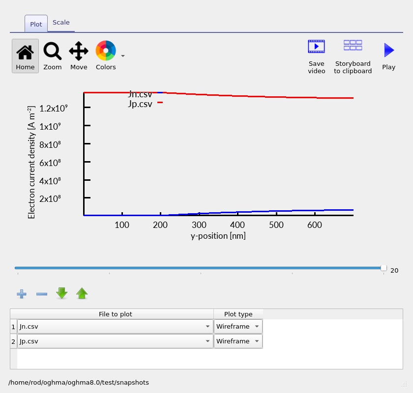
Small-current plots can be numerically delicate. Assess the overall trend and current continuity rather than attributing every narrow oscillation to a physical transport mechanism. If you encounter large deviations, refine the mesh and check solver convergence before drawing conclusions.
6.4 Radiative and SRH recombination
Inspect R_nfree_to_pfree.csv (free-to-free radiative recombination) and R_ss_srh.csv (single-level SRH recombination). The recombination screenshots (??) display these channels together. Under injection, the absolute recombination rate can increase strongly; its location is determined by the overlap of free carriers, the material properties and the chosen trap parameters.
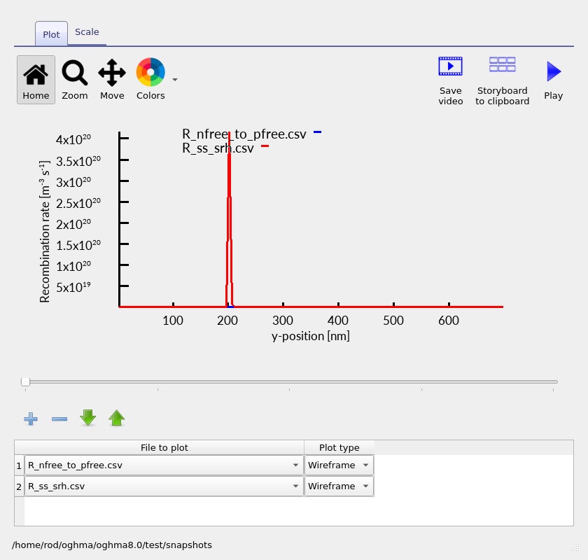
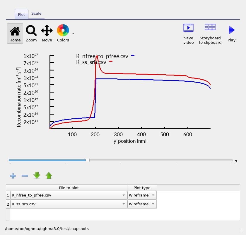
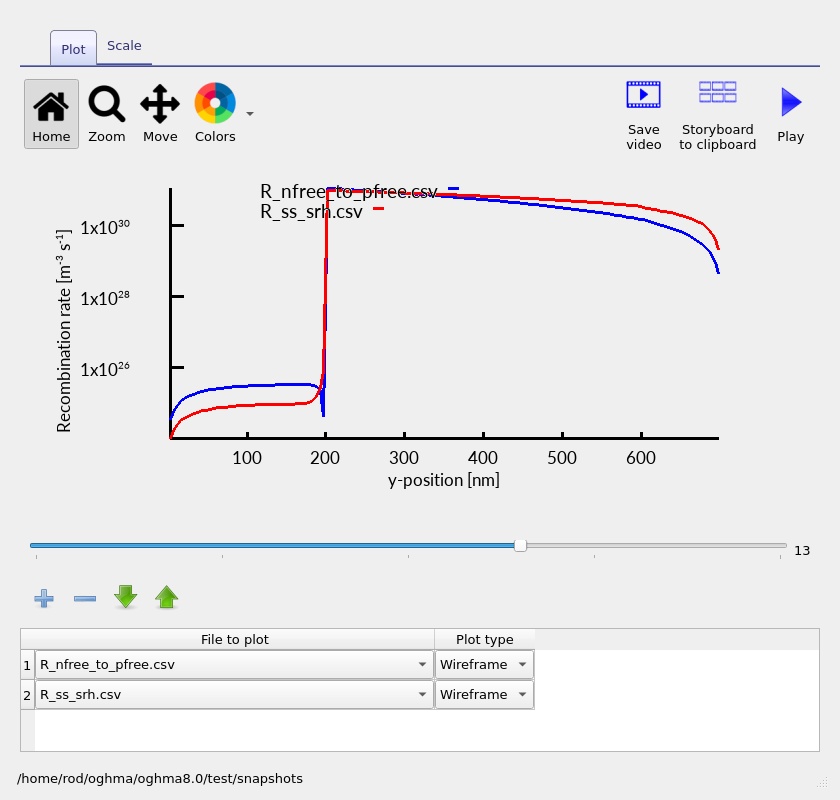
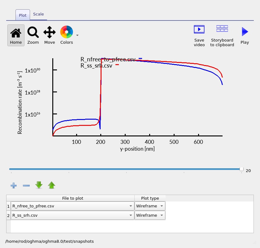
Watch especially for features at the p-AlGaAs/n-GaAs interface. A local feature can be physically meaningful, but its magnitude alone does not prove interface trapping: the present exercise uses bulk material models and the configured SRH parameters. Compare the integrated contribution and the spatial distribution of both processes before declaring a dominant loss mechanism.
6.5 Electron and hole rate profiles
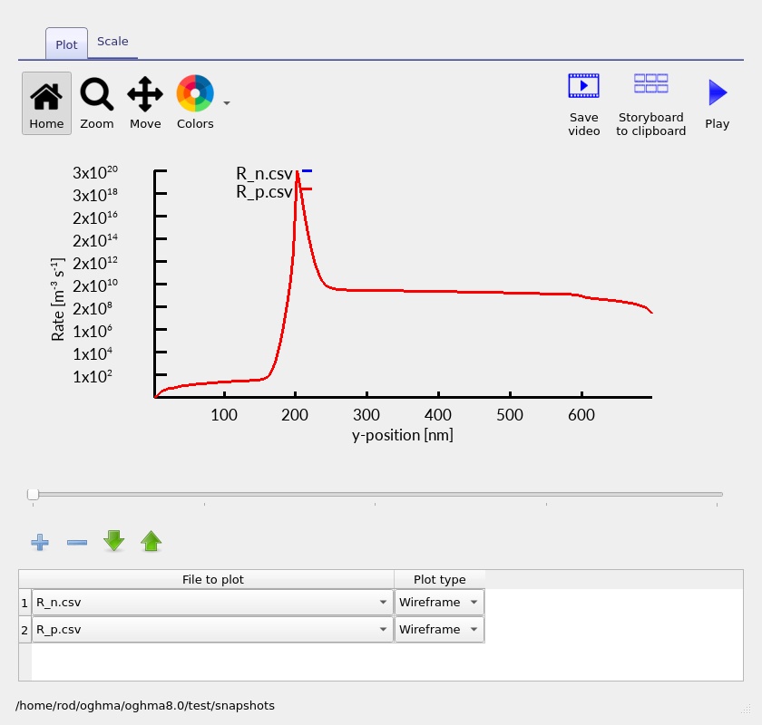
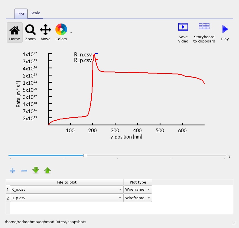
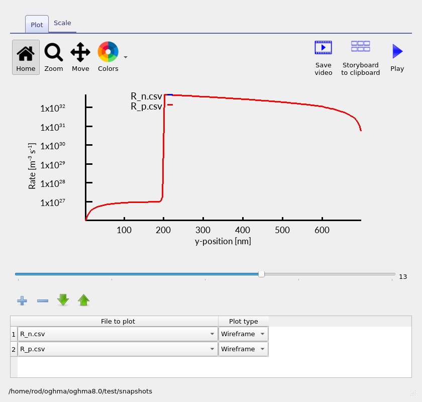
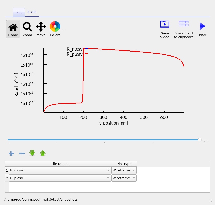
The separate R_n.csv and R_p.csv results expose the electron- and hole-related rate balances used in the simulation. These plots (??) provide an additional check on where carriers are removed or redistributed during the sweep. Interpret signs and plotted components according to their data headers rather than assuming all curves represent a single positive recombination rate.
6.6 Carrier mobilities
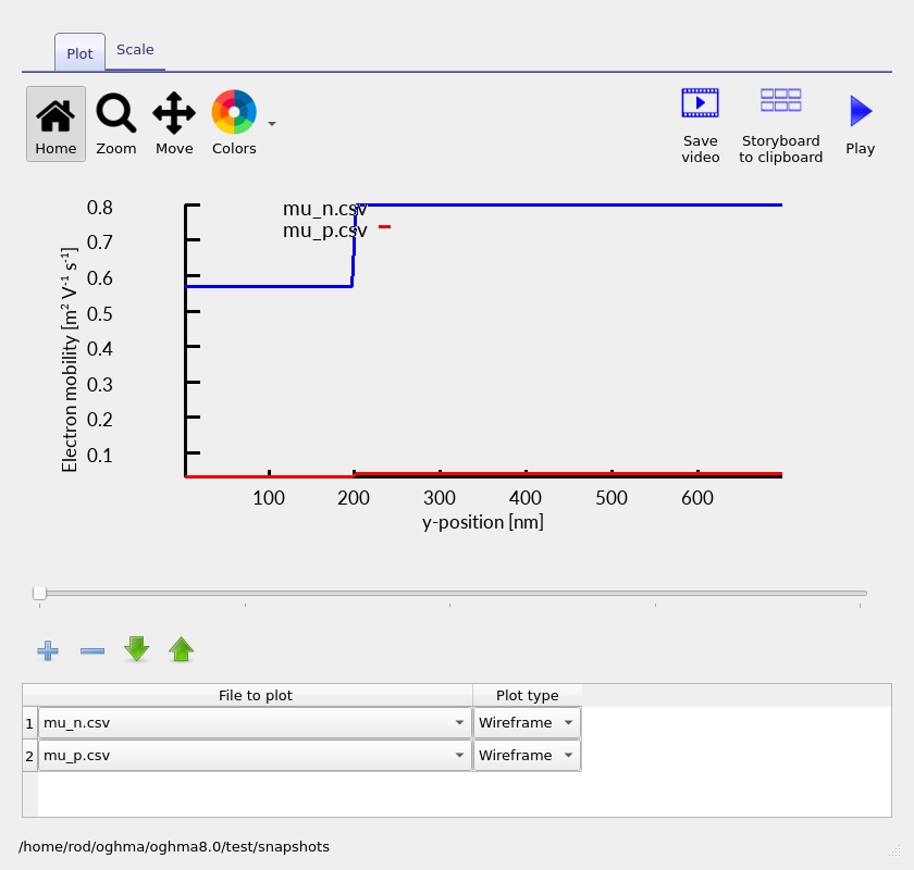
The mobility output provides a way to inspect transport parameters as a function of position. Changes across the interface are expected because the AlGaAs and GaAs models need not return the same mobility. The example mobility screenshot (??) shows one saved viewer position; it is not evidence for a particular field-dependent mobility effect.
7. Exercises: connecting band offsets to diode behaviour
8. Assumptions and limits of the example
This is an idealised 1D teaching example. The semiconductor thicknesses and doping concentrations are plausible for an epitaxial III–V stack, but the example does not by itself establish a manufacturable or performance-optimised product. The calculation assumes idealised ohmic contacts, a laterally uniform structure, an abrupt material interface and the transport/recombination physics supplied by the selected models.
The AlGaAs/GaAs interface may involve additional transport physics in real devices; practical contacts, defects, surface recombination, alloy disorder, self-heating and substrate effects can also alter measured characteristics. Auger recombination is switched off in this input, and the simulation is a dark electrical sweep, not a calibrated LED, photodiode or solar-cell efficiency prediction. Quantitative validation requires experimental data and independently checked material parameters.
9. Next steps
Having reproduced the J–V curve and located the heterojunction in the band diagram, the most informative next calculation is a controlled alloy-composition comparison: vary the aluminium fraction, keep doping and thickness fixed, and track the conduction-band step, valence-band step and forward-bias current. A GaAs homojunction run provides a useful reference.
For more detail about how OghmaNano stores device configuration and material-model parameters, see the advanced Oghma file format documentation.