

GaN PIN Diode Simulation: Drift–Diffusion, J–V Curves and Wide-Bandgap Transport
1. Introduction
A gallium nitride (GaN) PIN diode is a wide-bandgap semiconductor device with a p-type region, a comparatively lightly doped (nominally intrinsic) region and an n-type region. Unlike an ordinary PN junction, a PIN diode deliberately introduces a substantial drift region between the doped terminals. Under reverse bias, this region can support a distributed electric field; under forward bias, injected electrons and holes allow the structure to conduct. These properties make the PIN architecture relevant to the underlying principles of power rectification, reverse-voltage blocking and wide-bandgap device engineering.
GaN has a room-temperature bandgap of approximately 3.4 eV and can sustain high electric fields compared with silicon. Practical GaN power diodes nevertheless require careful control of drift-layer thickness and background doping, contact resistance, crystal defects and edge termination. The 800 nm intrinsic-GaN region in this example is deliberately compact: it makes the central electrostatics and carrier injection straightforward to explore, but does not by itself represent a rated high-voltage power rectifier.
This tutorial uses OghmaNano's coupled Poisson and drift–diffusion equations to solve a one-dimensional GaN PIN diode. Rather than treating current as a single circuit quantity, the model resolves the internal band profile, quasi-Fermi levels, electron and hole concentrations and recombination rates as bias is changed. The aim is to connect an intuitive rectifying J–V curve to the physical processes taking place inside the semiconductor.
2. Making a new simulation
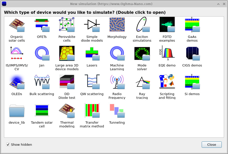
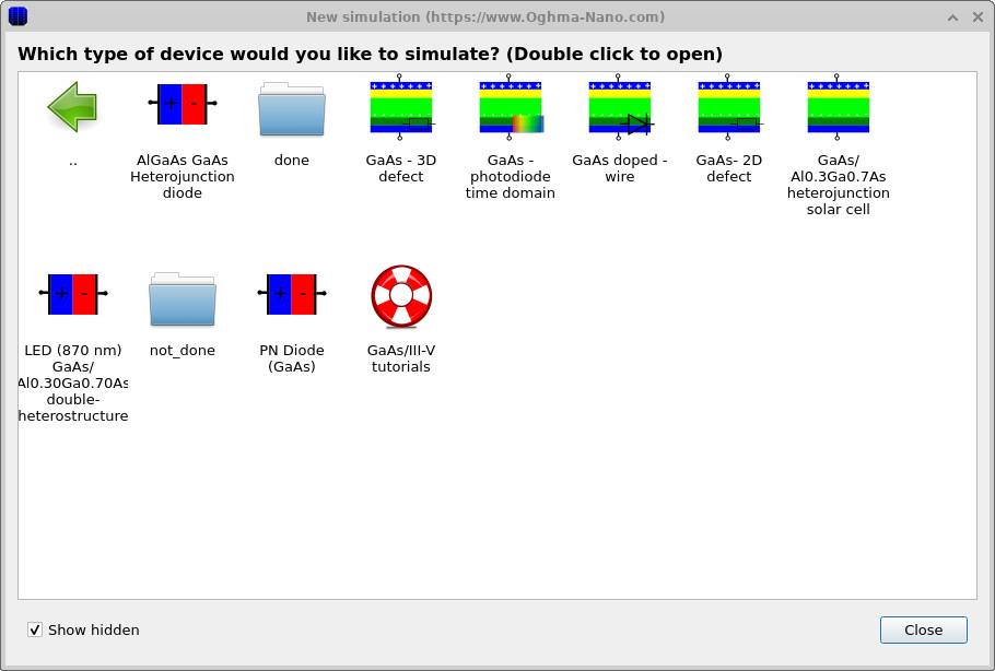
Open OghmaNano and select New simulation. Choose the III–V semiconductor demonstrations and open the GaN PIN diode example. The available simulation categories and demonstration-selection window are shown in Figures ?? and ??. If the demonstration is already installed, opening it should display the layer stack in the main device window.
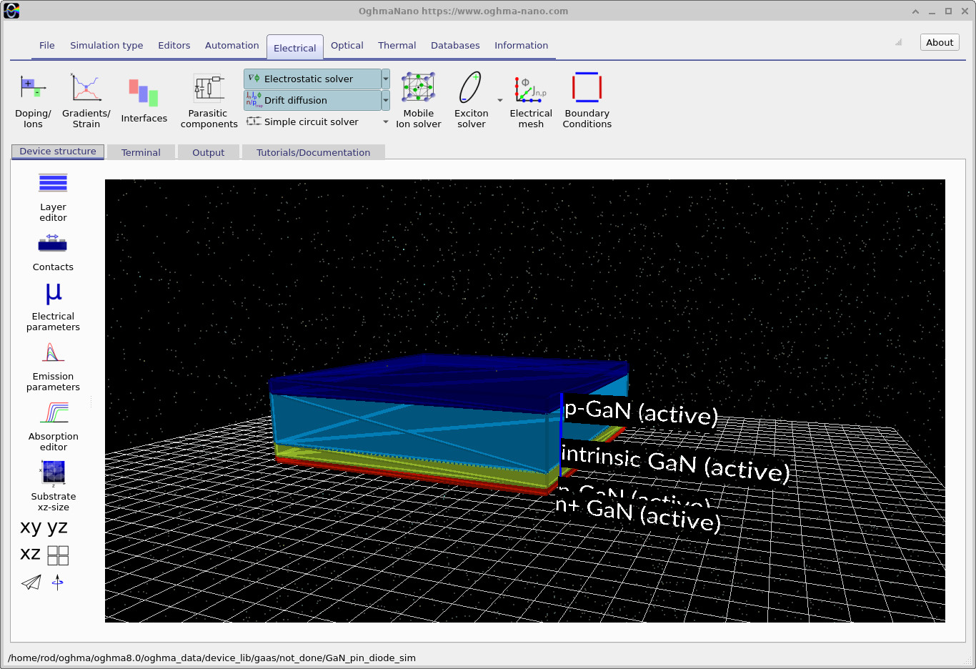
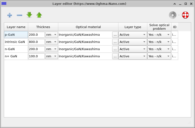
The main simulation view (??) shows a three-dimensional representation of the device. Although the visualisation is 3D, the numerical example presented here resolves electrical transport along the layer-growth direction only. Open the Layer editor to see the actual thickness and material assignment for each region.
3. Layer structure and doping
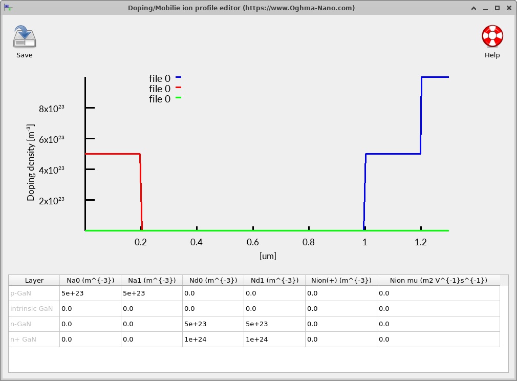
The completed demonstration uses the following electrically active semiconductor structure. The 800 nm intrinsic layer is the configuration used for the simulation illustrated here; older copies of the example may contain a 400 nm intrinsic layer and should be updated before attempting to reproduce these results.
| Layer | Thickness | Nominal dopant concentration | Purpose |
|---|---|---|---|
| p-GaN | 200 nm | Acceptors: 5 × 1017 cm−3 | p-side injection and anode region |
| Intrinsic GaN | 800 nm | No intentional doping | Lightly doped drift and depletion region |
| n-GaN | 200 nm | Donors: 5 × 1017 cm−3 | n-side junction region |
| n⁺-GaN | 100 nm | Donors: 1 × 1018 cm−3 | Back-contact region |
The active semiconductor stack is 1.3 µm thick. A separate 200 nm air region may appear in the layer editor for the device visualisation and optical geometry; it is not part of the electrically active PIN stack. All four semiconductor regions use GaN, so the purpose of the interfaces here is to change doping, not semiconductor alloy composition.
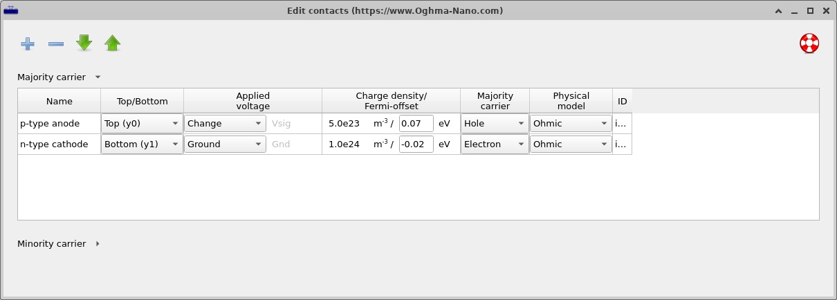
Open the Contacts editor (see the figure below) to inspect the anode and cathode, then open the Doping editor (see the figure below). The acceptor-doped p region and donor-doped n/n⁺ regions should appear on opposite sides of a wide undoped central region. The centre of the structure is not a separate material heterojunction: its principal distinguishing feature is low intentional doping.
In the idealised depletion approximation, a low-net-charge drift region can support an electric field that extends across much of its thickness. The voltage supported by a region is related to the spatial integral of its electric field:
\[V_{\mathrm{region}}=-\int_{y_0}^{y_1} E(y)\,\mathrm{d}y.\]Thus, a wider lightly doped region can distribute an applied reverse potential over a larger distance. This is a central reason PIN structures are investigated for voltage blocking. It does not mean the breakdown voltage can be obtained simply by multiplying thickness by an assumed critical field: real devices have nonuniform fields, background charge, contacts and field crowding at edges.
4. Electrical models, contacts and numerical configuration
4.1 GaN material parameters
Open the electrical parameter editor to inspect the transport and recombination settings used for each GaN region. The simulation is configured to load GaN properties from the OghmaNano material database, with the relevant database-override flags disabled. This is preferable to assigning arbitrary effective mobilities, bandgaps or electron affinities in the device JSON. Check the loaded material data if you need a quantitatively reproducible comparison with experiment.
For GaN, the principal considerations include the wide bandgap, the electron and hole mobilities, free-carrier statistics, radiative recombination and trap-assisted recombination. The nominal acceptor concentration shown in the doping editor should not automatically be identified with the free-hole density: Mg acceptors in p-GaN are incompletely ionised at room temperature. The extent to which the electrical model handles dopant ionisation should be considered before assigning a physical contact resistance or extracting a measured carrier density.
4.2 Contacts and boundary conditions
The demonstration uses ideal ohmic contacts for the p-side anode and n-side cathode. These simplify interpretation by avoiding a second rectifying element at a metal/semiconductor interface. In fabricated GaN devices, especially at p-GaN contacts, attaining low-resistance ohmic behaviour can be challenging and involves the metal stack, surface preparation and doping.
4.3 Electrical mesh
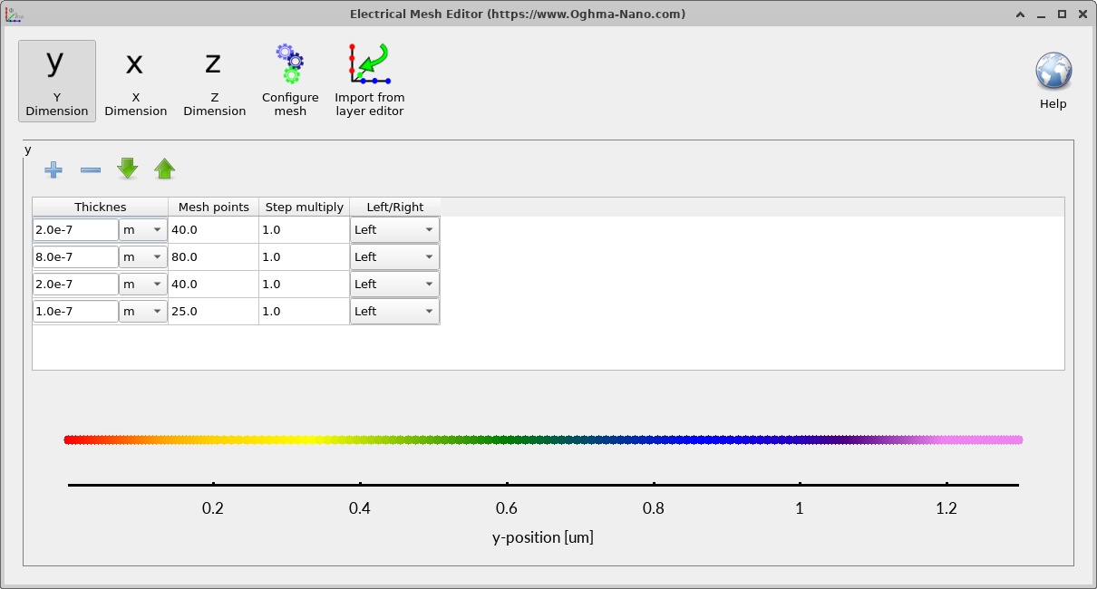
The Electrical mesh editor (shown below) shows the discretisation along the semiconductor thickness. When changing the intrinsic region from 400 nm to 800 nm, ensure that the mesh covers the updated 1.3 µm active stack. A starting choice of approximately 250–260 points gives spacing on the order of 5 nm; the software may remesh automatically depending on the configuration. For a more quantitative study, repeat the simulation with a finer mesh and check that the J–V curve and internal profiles remain effectively unchanged.
4.4 Transport and recombination
OghmaNano couples the electrostatic Poisson equation to electron and hole continuity equations. In one dimension the steady-state equations may be written schematically as
\[\frac{\mathrm{d}}{\mathrm{d}y}\!\left(\varepsilon\frac{\mathrm{d}\phi}{\mathrm{d}y}\right)=-\rho,\qquad \frac{\mathrm{d}J_n}{\mathrm{d}y}=q(R-G),\qquad \frac{\mathrm{d}J_p}{\mathrm{d}y}=-q(R-G),\]where \(\phi\) is the electrostatic potential, \(\rho\) the local space-charge density, \(J_n\) and \(J_p\) the electron and hole current densities, \(G\) the generation rate and \(R\) the net recombination rate. With these sign conventions the total current density \(J_n+J_p\) is constant through a converged, steady-state one-dimensional device.
The recombination model may contain direct band-to-band (free-to-free) and Shockley–Read–Hall (SRH) contributions. Their relative importance depends on material quality, injection level and the model parameters. GaN's direct bandgap makes radiative recombination physically possible, but its presence in a model does not imply that a particular plotted device is an efficient LED.
5. Running the dark J–V simulation
Set the voltage sweep to −2.0 V to +5.0 V in increments of 0.025 V. Negative voltage reverse-biases the PIN structure and positive voltage drives it into forward conduction. The intended bias configuration is:
"Vstart": -2.0,
"Vstop": 5.0,
"Vstep": 0.025
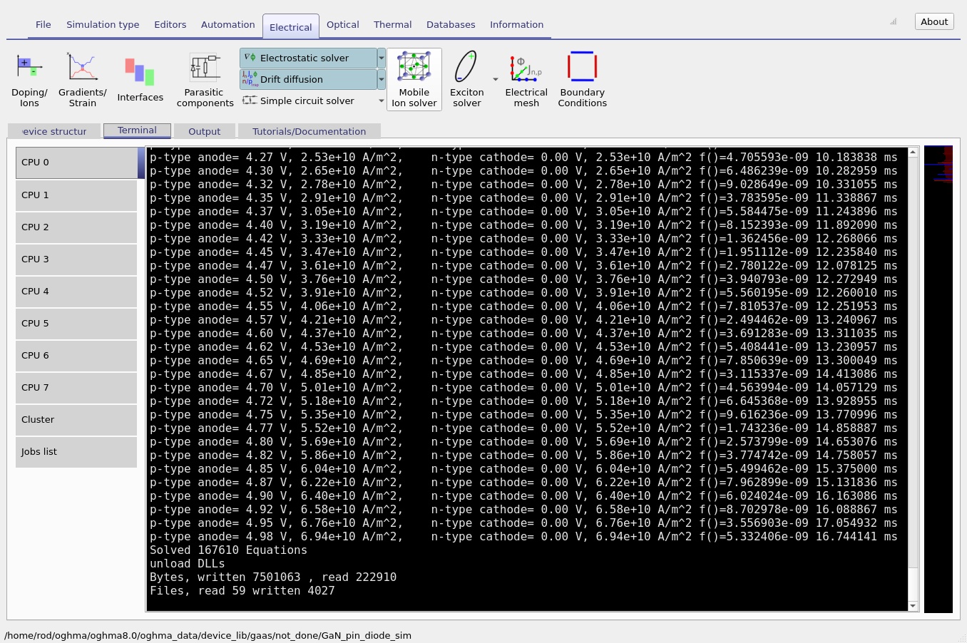
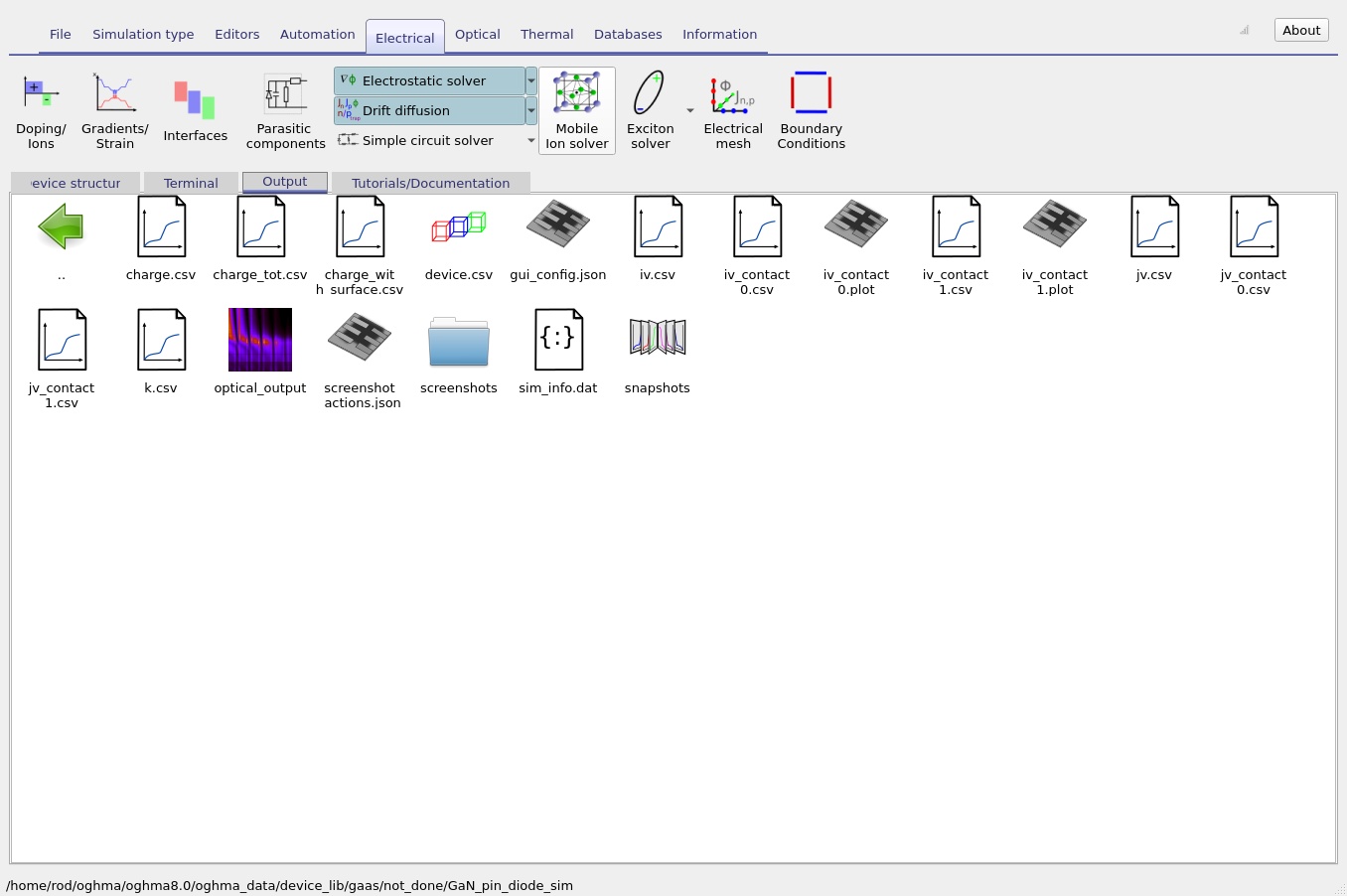
From the main window select Run simulation. While the calculation runs, use the Terminal tab to monitor progress and convergence. After completion, open the Output tab and select jv.csv to plot the current density against applied voltage. The output browser, solver terminal and resulting J–V curve are shown below.
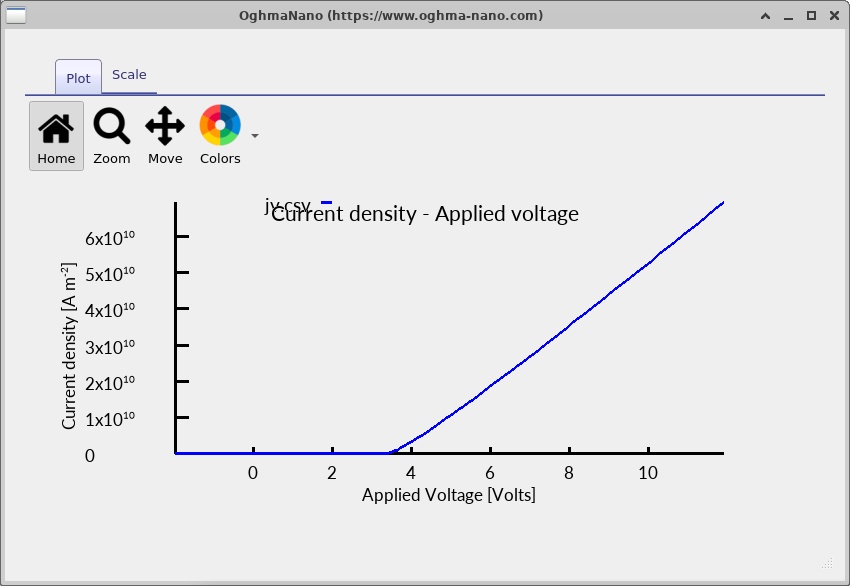
At reverse bias the simulated current is small relative to its forward-bias value. As the positive bias is increased, carrier injection rises rapidly and the diode turns on. At larger forward voltages the curve becomes more nearly linear on a linear current-density axis, indicating that the current is increasingly influenced by resistive transport and other non-idealities in the simulated structure. A flattening slope on a logarithmic current axis should not automatically be interpreted as hard current saturation: a roughly linear current increase also appears progressively flatter on a log plot.
For a simple comparison with diode theory, the low-to-moderate forward-bias characteristic can be related to
\[J\approx J_0\left[\exp\!\left(\frac{qV}{nk_{\mathrm B}T}\right)-1\right],\]where \(J_0\) is an effective saturation current and \(n\) an effective ideality factor. A PIN diode may depart substantially from a single ideal Shockley regime because depletion-region recombination, injection into the intrinsic layer, high-level injection and series resistance can influence the current. The simple expression should therefore be regarded as a diagnostic approximation rather than the governing equation solved by OghmaNano.
Reverse-voltage blocking is not equivalent to demonstrated avalanche breakdown. A sweep down to −2 V tests the small-reverse-bias behaviour only. The voltage at which a fabricated GaN power device breaks down depends on high-field physics, material defects, leakage paths, geometry and edge termination, and cannot be inferred from this demonstration alone.
6. Examining the internal simulation results
After the J–V sweep, OghmaNano's snapshot viewer allows spatially resolved results to be plotted at selected bias points. The screenshots below illustrate four positions in the stored sweep, running from the earliest to the latest selected snapshot. Their names (-0 to -3) identify screenshot positions, not voltages. Read the actual selected voltage from the snapshot viewer when making quantitative comparisons.
6.1 Band edges and quasi-Fermi levels
Open the snapshot viewer and plot Ec.csv, Ev.csv, Fn.csv and Fp.csv together. These correspond to conduction- and valence-band edges and the electron and hole quasi-Fermi levels. Figures ??–?? show their evolution through the bias sweep.
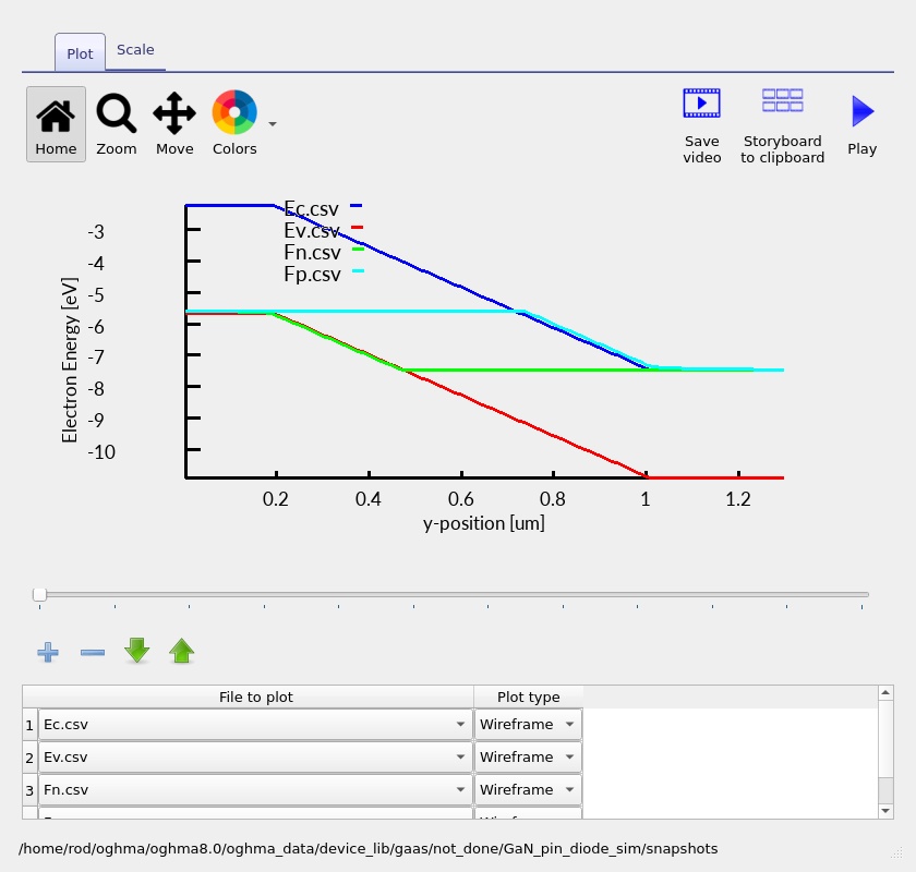
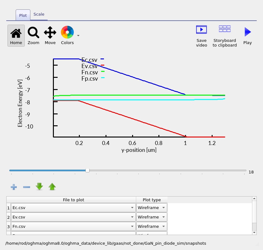
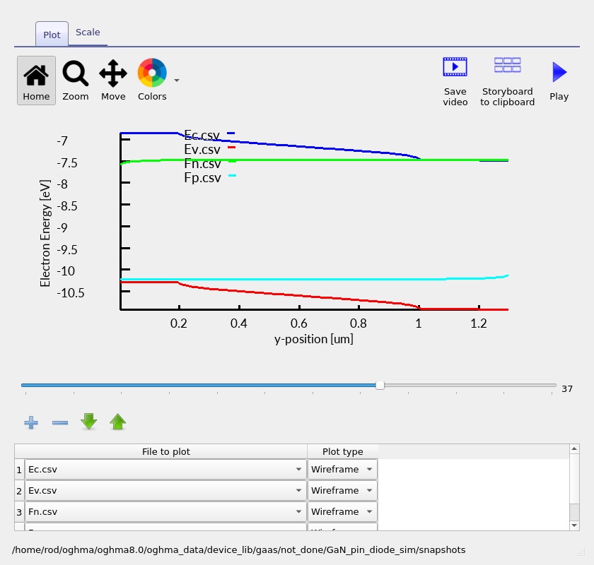
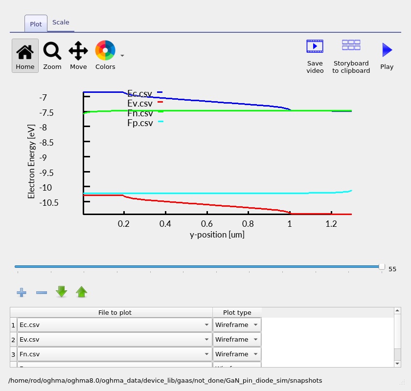
In reverse bias, much of the potential variation is expected to occur across the lightly doped intrinsic region, producing a relatively extended band slope. Forward bias reduces the effective injection barrier and creates a bias-dependent separation of electron and hole quasi-Fermi levels. The spatial gradients of these levels are important because they determine current flow; band bending and quasi-Fermi splitting should be considered together rather than interpreted independently.
As a basic physical check, the separation between \(E_c\) and \(E_v\) in the GaN layers should be consistent with the material database's GaN bandgap, rather than a leftover default value from another semiconductor. Since this is a homomaterial PIN device, abrupt composition-induced band offsets are not expected at the p/i/n transitions.
6.2 Electron and hole densities
Plot Q_nfree.csv and Q_pfree.csv (or the electron and hole carrier-density results presented by your installed version). At low injection the majority-carrier densities are concentrated in their respective doped regions. The undoped central region contains much lower equilibrium carrier concentrations. In strong forward bias, injected carriers populate a larger fraction of the intrinsic region and recombination can increase substantially.
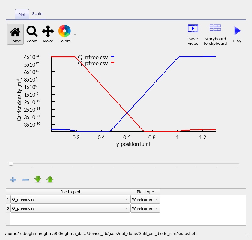
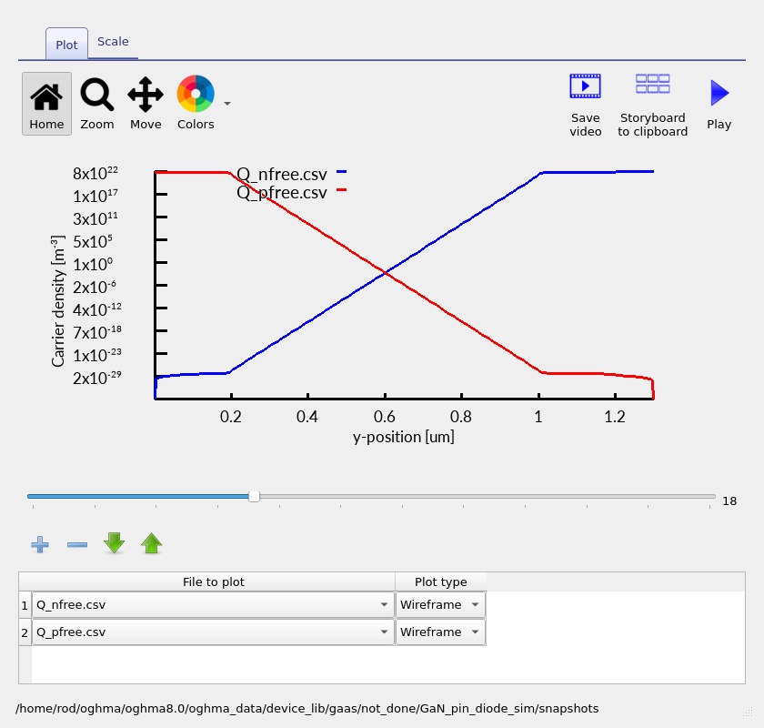
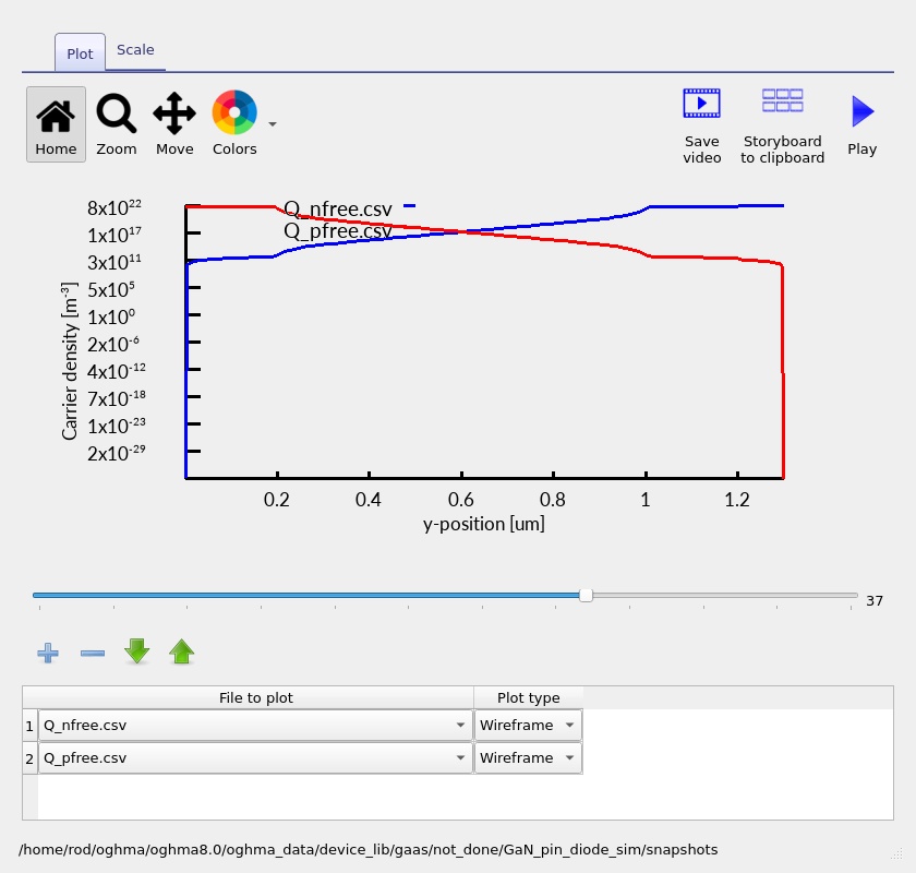
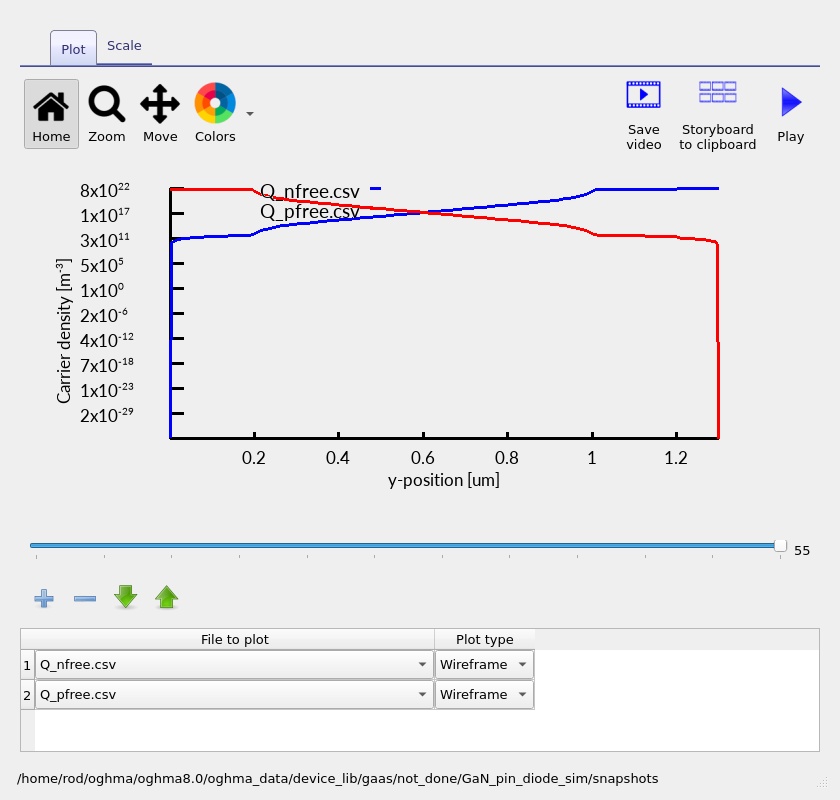
The abrupt change in nominal dopant density does not imply an identical abrupt free-carrier profile. Carrier density is determined self-consistently from the band energies, Fermi levels, density of states and charge neutrality. This is especially relevant on the p-GaN side if the material model uses a simplified treatment of incomplete acceptor ionisation.
6.3 Recombination in the intrinsic region
View the spatial recombination plots at the same bias points. The recombination figures in this example show how the region of significant electron–hole overlap and recombination develops as forward injection increases. Interpret the height and width of each plotted profile together: a large local peak is not necessarily the largest contribution to the device-integrated recombination rate.
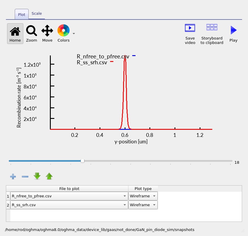
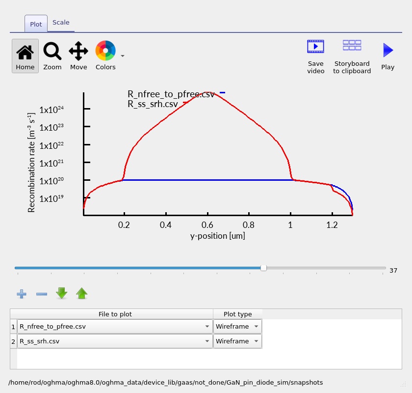
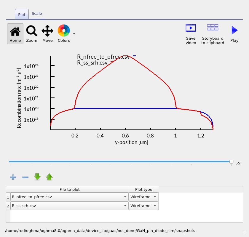
For a direct band-to-band process, the net radiative rate commonly follows the form
\[R_{\mathrm{rad}}=B\left(np-n_i^2\right),\]where \(B\) is the material recombination coefficient. SRH recombination depends on defect parameters and can show a different spatial distribution. To compare mechanisms, plot them separately if both are available and enabled in the loaded device. Do not assume that an unlabeled total recombination plot identifies a single microscopic mechanism.
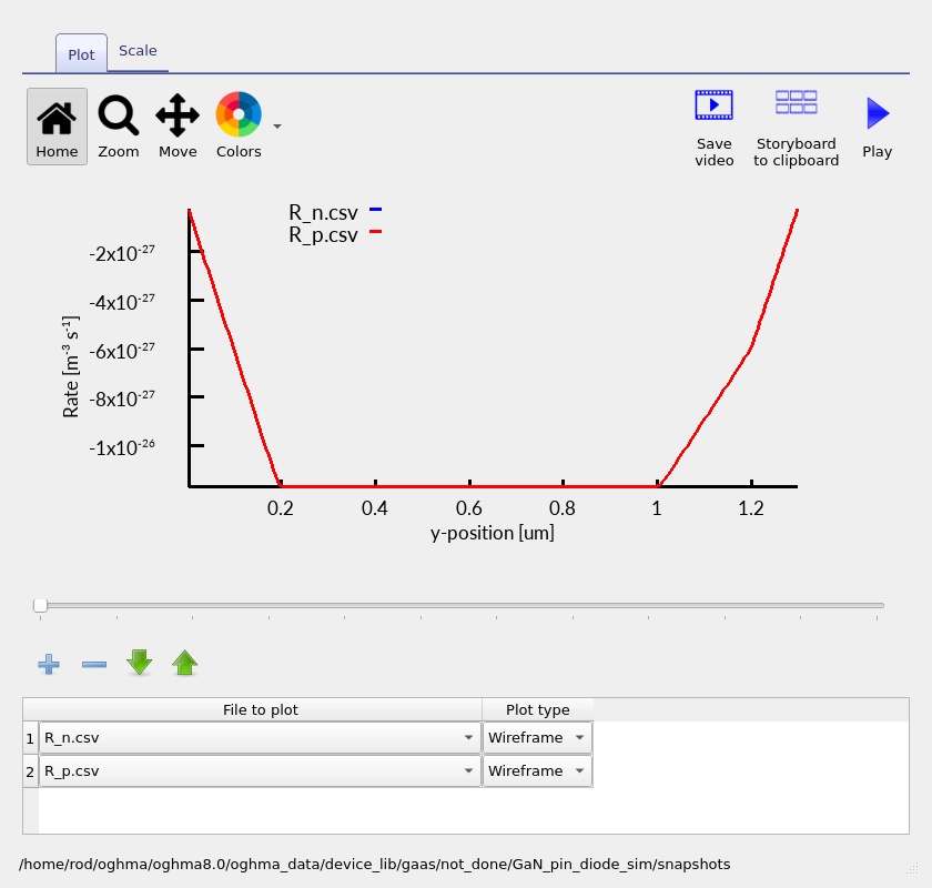
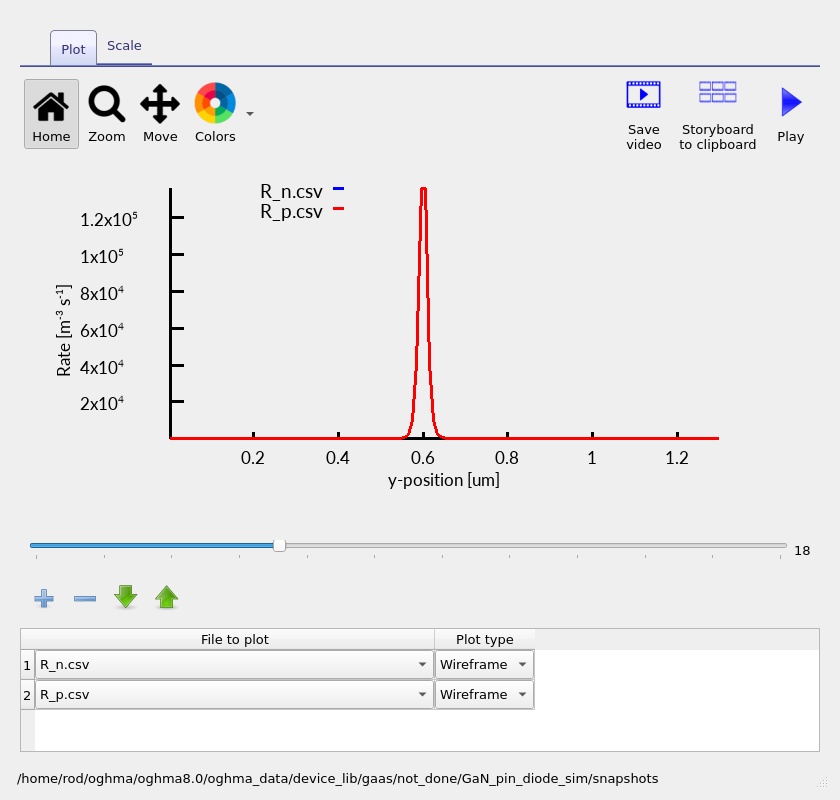
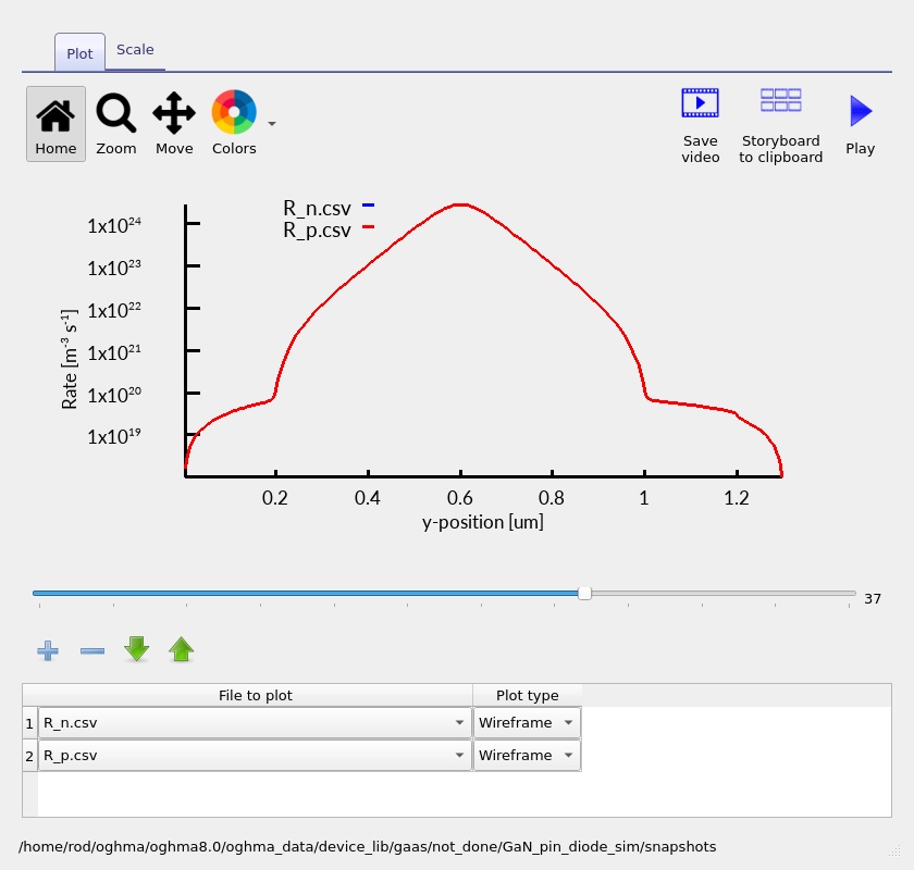
6.4 Electron and hole recombination/continuity rates
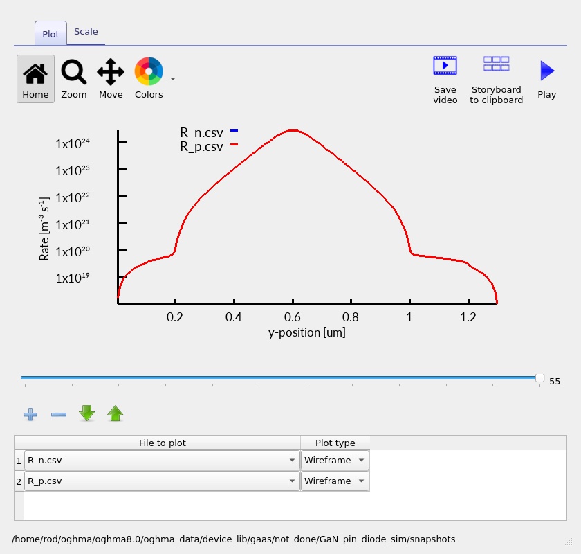
The additional electron- and hole-rate plots are useful for examining where carrier populations change most rapidly through recombination and injection. The four screenshots below show how these calculated profiles change with bias. If the displayed rate is signed or contains both generation and recombination contributions, use the plot legend and data-file header to determine the correct physical interpretation before comparing magnitudes.
6.5 Current conservation as a model check
For any steady-state bias point, plot the electron current density \(J_n\) and hole current density \(J_p\) if those outputs are available. Each component can change with position as carriers recombine, but the total \(J_n+J_p\) should be spatially conserved in a converged 1D device without additional charge-accumulation terms. This is a particularly helpful check when a small apparent ripple in a low-current trace might otherwise be mistaken for a physical effect.
7. Suggested exercises
8. Physical assumptions and limitations
This example is intended as an educational bulk GaN drift–diffusion simulation. It provides a physically meaningful first look at PIN electrostatics and carrier injection, but it is not a calibrated commercial device model. In particular, the results should be interpreted with the following qualifications.
- Idealised contacts: the metal/GaN contact barriers and practical p-GaN contact resistance are not explicitly validated.
- Nominal doping: p-type acceptor activation and background residual charge in nominally intrinsic GaN can change the physical charge distribution.
- High-field breakdown: the J–V sweep does not determine avalanche breakdown, termination-limited blocking voltage or reliability under high reverse bias.
- One-dimensional transport: the model omits lateral current crowding, edge leakage, field plates and device termination geometry.
- Defects and recombination: realistic quantitative leakage and recombination predictions require calibrated bulk and interface defect parameters.
- Thermal and dynamic effects: self-heating, switching transients and minority-carrier charge-storage effects must be assessed separately when relevant.
These limitations do not diminish the value of the example as a starting point. The layer stack and J–V curve illustrate what happens when a low-doped drift region is inserted into a wide-bandgap semiconductor diode. They also provide a reproducible baseline for testing more advanced transport and recombination models.
9. Next steps
Having examined the GaN PIN diode, compare its field distribution with an ordinary GaN PN junction and then investigate how intrinsic-layer thickness and residual doping influence rectification. More advanced work could introduce calibrated trap states, non-ideal contacts and high-field transport mechanisms to examine the limits of the simple drift–diffusion picture.