

GaN PN Junction Diode Simulation: Drift–Diffusion, J–V Curves & Recombination
1. Introduction
A gallium nitride (GaN) PN junction diode consists of p-type and n-type regions of the same semiconductor, brought together to form a rectifying junction. Electrons and holes redistribute across the interface, producing a depletion region and a built-in potential barrier. Under forward bias, the barrier is reduced and the current rises sharply; under reverse bias, the junction suppresses carrier injection. The resulting asymmetric current–voltage response is the basic operating principle of a semiconductor rectifier.
GaN is a wide-bandgap III–V semiconductor, with a room-temperature bandgap of approximately 3.4 eV. Its high critical electric field and low intrinsic carrier concentration make it attractive for power conversion, electrical rectification and high-temperature electronics. The compact p-GaN/n-GaN homojunction in this tutorial provides a clear way to investigate how the built-in barrier controls current flow and how GaN's material properties influence a rectifying junction.
In this tutorial, OghmaNano is used to explore electrical rectification, drift–diffusion carrier transport, band bending and recombination. Its coupled Poisson and electron/hole continuity equations calculate the current flowing through the diode together with the internal carrier and electrostatic profiles as a function of position and applied voltage. This links the familiar J–V characteristic to the physical processes occurring across the junction.
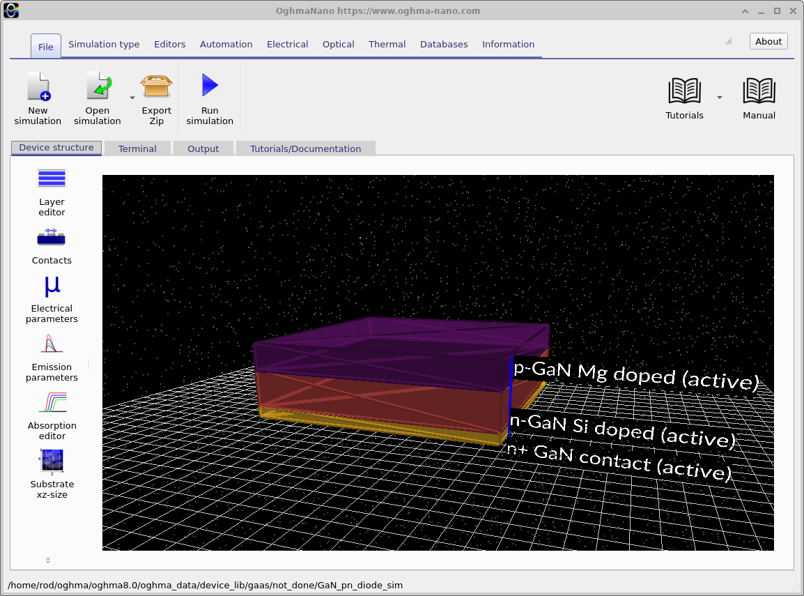
The thin, vertically stacked layers are displayed in the main OghmaNano device window (??). The visualisation is three-dimensional, but the electrical simulation presented here is one-dimensional along the layer-growth direction.
2. Making a new simulation
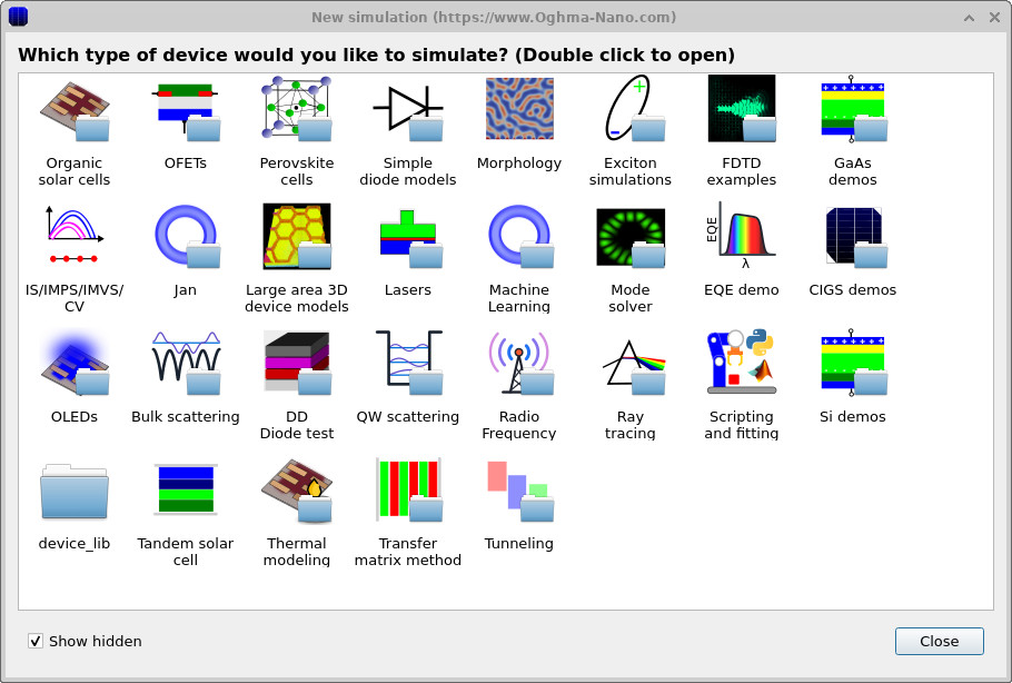
From the OghmaNano main window, select New simulation. The first dialog shows the available simulation categories (??). Open the III–V/GaN examples and select the GaN PN diode demonstration (??). The exact ordering of examples may differ between versions of OghmaNano.
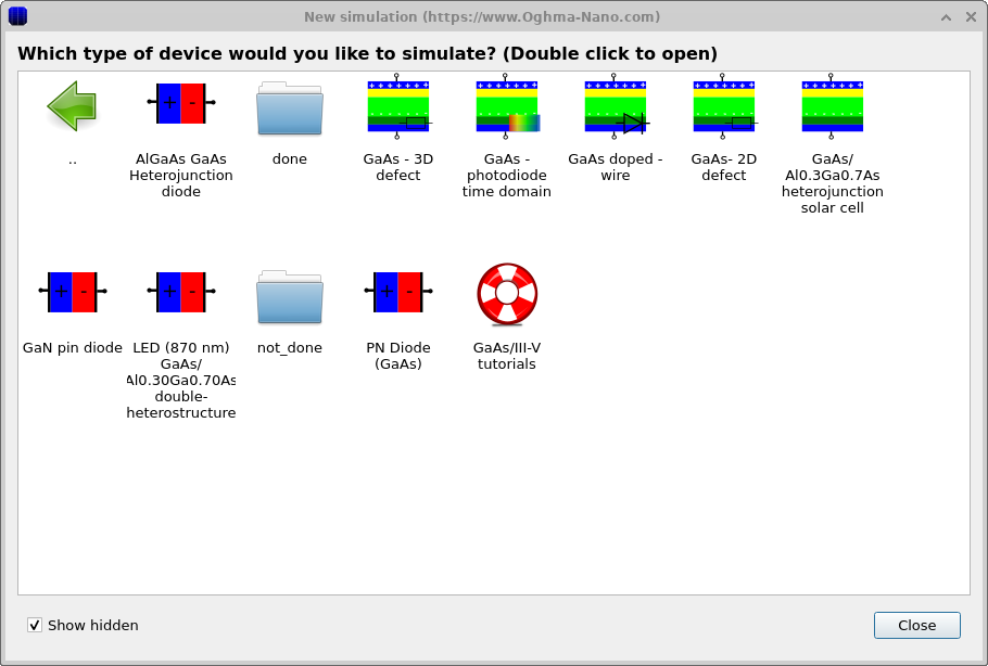
After loading the example, open the Layer editor from the device ribbon. This exposes the semiconductor regions, their thicknesses and the selected material database entries. The device is a PN homojunction, with the p-GaN and n-GaN layers forming the electrically active junction.
3. Examining the device structure, contacts and doping
3.1 Layer structure
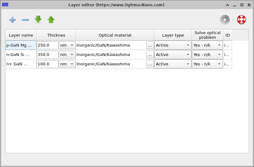
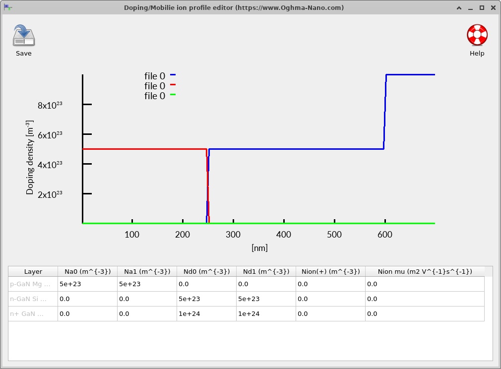
The electrical stack comprises three GaN regions. The p-GaN and n-GaN layers form the rectifying junction; the n⁺-GaN layer provides a more heavily doped region adjacent to the cathode. The total semiconductor thickness is 700 nm, excluding the surrounding air used for visualisation. The layer editor is shown in ??.
| Layer | Thickness | Nominal doping | Electrical role |
|---|---|---|---|
| p-GaN (Mg-doped) | 250 nm | \(N_A=5\times10^{17}\,\mathrm{cm^{-3}}\) | Hole-majority side of the PN junction |
| n-GaN (Si-doped) | 350 nm | \(N_D=5\times10^{17}\,\mathrm{cm^{-3}}\) | Electron-majority side of the PN junction |
| n⁺-GaN | 100 nm | \(N_D=1\times10^{18}\,\mathrm{cm^{-3}}\) | More heavily doped cathode-side region |
3.2 Contacts
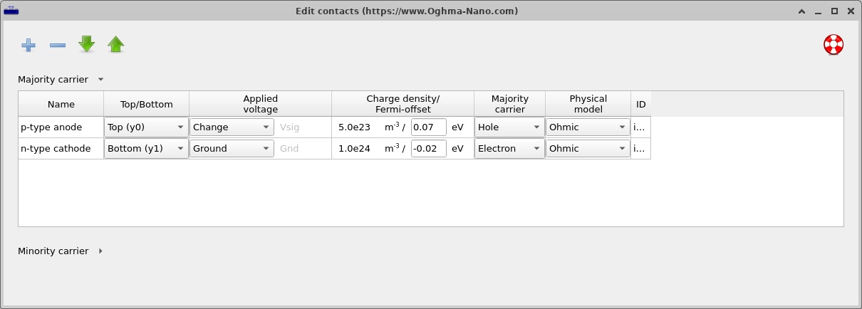
The example uses ideal ohmic boundary conditions at its p-side anode and n-side cathode. These boundary conditions make it possible to focus on the junction's internal electrical response. In fabricated GaN diodes, contact resistance and Mg acceptor activation influence the voltage drop and current injection; both are useful parameters for more advanced studies.
3.3 Doping profile and depletion region
Open the Doping / Ions editor from the Electrical ribbon to view the acceptor and donor distributions (??). A single abrupt transition from acceptor-doped p-GaN to donor-doped n-GaN defines the active PN junction. The n⁺ region introduces a second step in donor concentration near the cathode.
At thermal equilibrium the junction develops a depletion region as mobile carriers diffuse and leave behind ionised dopants. Within the depletion approximation, the characteristic width depends on the permittivity, doping on each side and the potential supported by the junction. For a conventional abrupt junction, the familiar relationship is
\[ W \simeq \sqrt{\frac{2\varepsilon_s}{q}\left(\frac{1}{N_A}+\frac{1}{N_D}\right)(V_{\mathrm{bi}}-V)}. \]Here \(V\) is the applied junction voltage, \(V_{\mathrm{bi}}\) is the built-in potential and \(\varepsilon_s\) is the GaN permittivity. This expression provides a useful reference for interpreting the self-consistent electric field calculated by OghmaNano, especially when examining how doping and applied bias affect the junction.
4. Electrical parameters and material models
4.1 GaN Lua material model
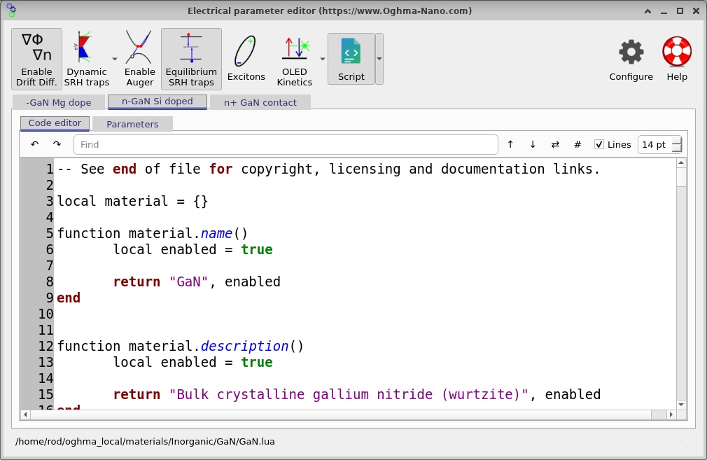
All three electrically active semiconductor layers reference the Inorganic/GaN/GaN.lua material model. The electrical material database supplies quantities such as the bandgap, electron affinity, density of states, permittivity, mobilities and recombination parameters. The JSON example has the relevant db_overrides switches disabled, so the operative numbers should be those returned by the Lua model rather than the dormant values visible elsewhere in the saved file. The GaN bandgap should be approximately 3.4 eV at room temperature; verify this in the displayed band profiles or the evaluated material parameters.
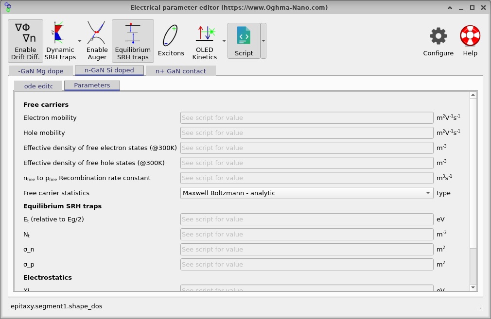
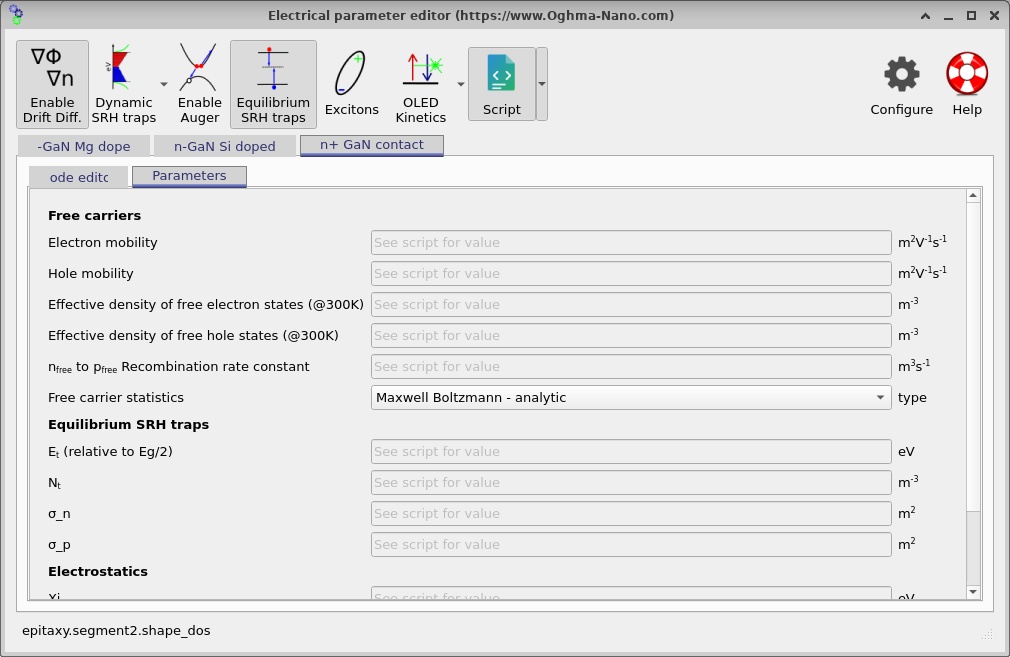
The screenshots for the material-code and parameter-editor views are grouped below. Some source screenshot filenames retain historical GaAs/AlGaAs labels; the active simulation described in this tutorial is GaN throughout. In the software, verify the GaN Lua material path rather than inferring the material from an image filename.
4.2 Carrier transport
OghmaNano solves the semiconductor Poisson equation together with electron and hole continuity equations, using drift–diffusion current expressions. The electron and hole current densities depend on the local field, mobility and carrier concentration gradient:
\[ J_n=q\mu_n n E+qD_n\frac{dn}{dy},\qquad J_p=q\mu_p p E-qD_p\frac{dp}{dy}. \]These expressions give two complementary mechanisms: drift due to the internal electric field and diffusion due to carrier concentration gradients. In steady state, their interplay determines the net diode current. The model also resolves the electron and hole quasi-Fermi levels, whose variation provides an alternative view of the carrier driving forces.
4.3 Recombination
Injected electrons and holes can recombine inside GaN. The example includes the material model's configured recombination processes, including defect-mediated Shockley–Read–Hall (SRH) terms where enabled by the effective material data. The usual idealised SRH expression is
\[ R_{\mathrm{SRH}}=\frac{np-n_i^2}{\tau_p(n+n_1)+\tau_n(p+p_1)}. \]The SRH lifetimes depend on trap densities, carrier thermal velocities and capture cross-sections. These parameters determine how efficiently injected carriers recombine and therefore influence the shape and magnitude of the current–voltage characteristic. Inspecting the spatial recombination rate helps identify where carrier loss is concentrated within the junction.
4.4 Numerical mesh
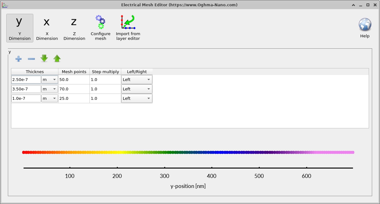
The electrical mesh spans the 700 nm GaN stack with 150 points along the growth direction, giving an average spacing of approximately 4.7 nm. This is a reasonable starting resolution for a teaching demonstration. The mesh editor (??) allows you to inspect the node distribution and refine it when investigating steep depletion-region gradients.
5. Running the J–V simulation
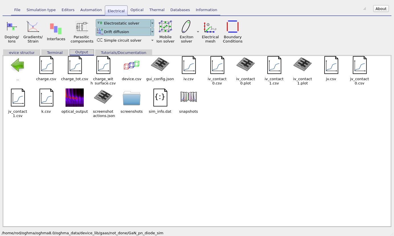
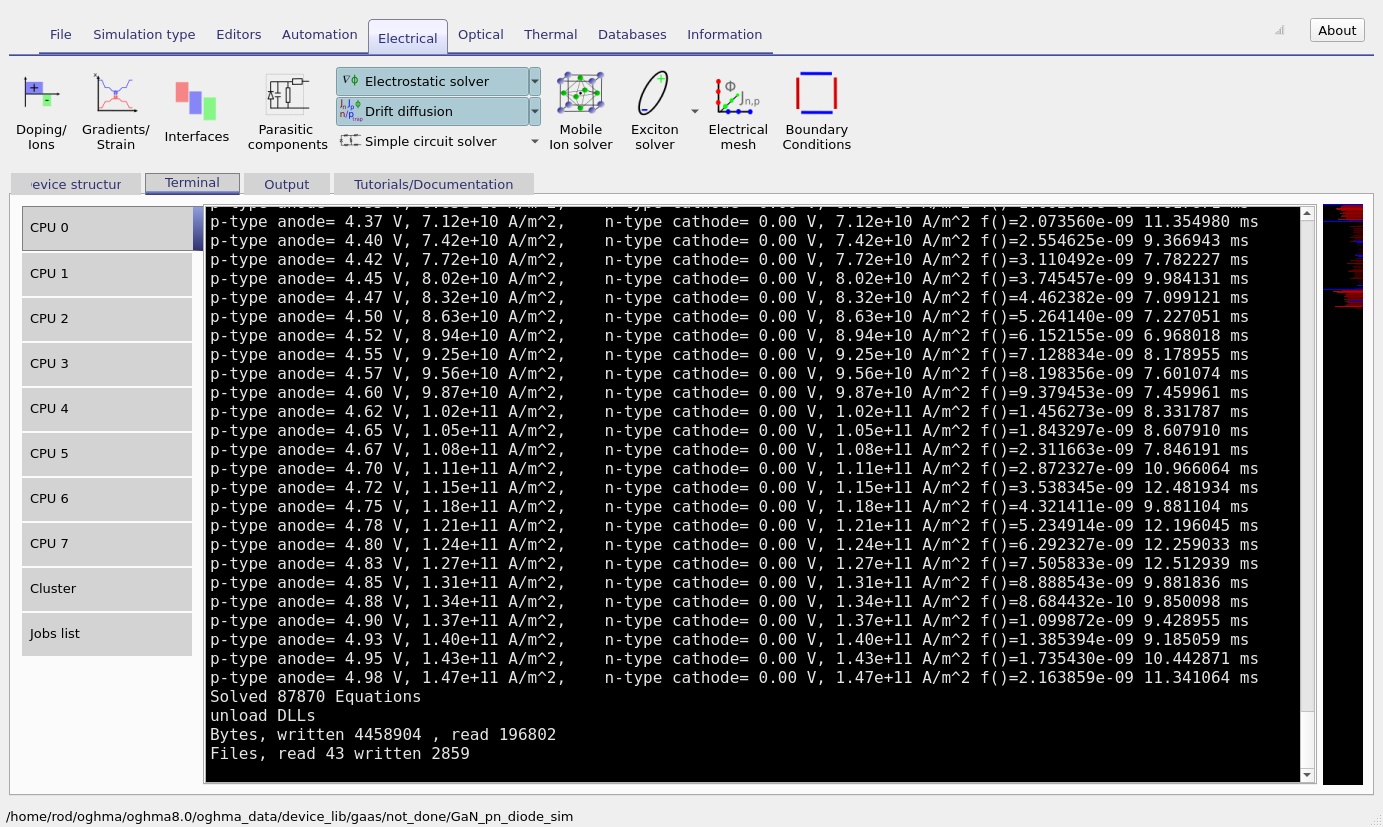
The example is configured for a voltage sweep from 0 V to +5 V in steps of 0.025 V. Start the simulation with the Run simulation control. During the sweep, the terminal window displays numerical progress and convergence information (??). After completion, the Output tab contains the generated results, including jv.csv and device-related data.
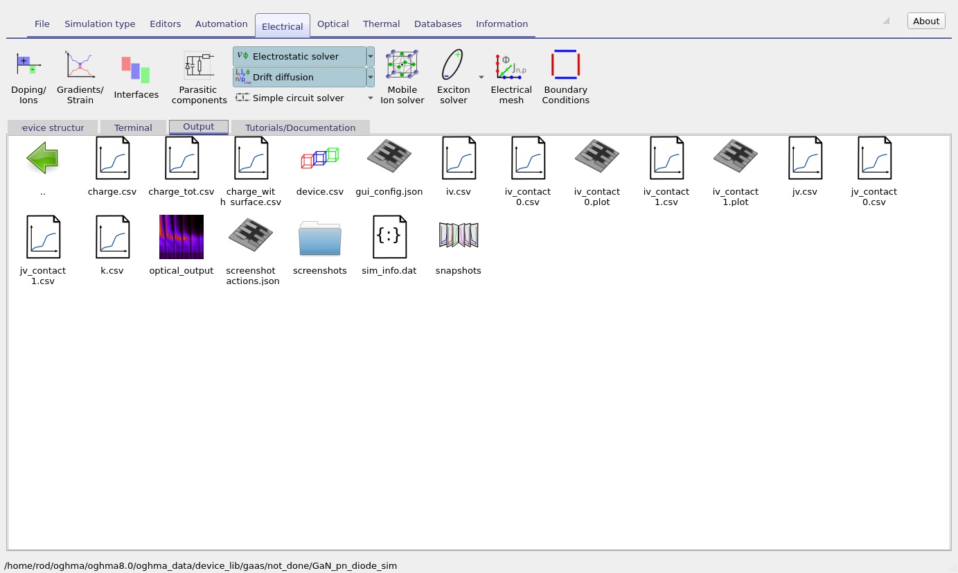
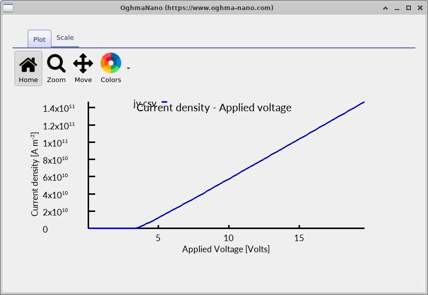
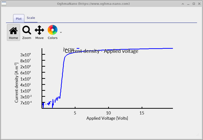
Open jv.csv to inspect the current density versus applied voltage. The linear view (??) and logarithmic view (??) present the same electrical response in complementary ways. The linear graph shows how current grows at high forward bias; the logarithmic graph makes the onset of injection and low-current response easier to resolve.
5.1 Interpreting the forward-bias curve
At low forward bias, the potential barrier strongly limits minority-carrier injection, so the net current remains small. As the applied voltage increases, the junction barrier decreases, electrons and holes cross the PN junction more readily and the current grows rapidly. On a semilogarithmic plot, a near-exponential region is often described locally using the diode equation
\[ J\simeq J_0\left[\exp\left(\frac{qV}{n_{\mathrm{id}}k_{\mathrm B}T}\right)-1\right], \]where \(J_0\) is an effective saturation current and \(n_{\mathrm{id}}\) is the ideality factor. This equation is a useful interpretation tool, not an independent model of the entire simulated device. In particular, a change in slope at higher current can reflect series resistance, injection effects or recombination changes. The strong current rise shown in the supplied screenshots is consistent with forward-bias rectification, but a specific ideality factor should only be quoted after fitting an appropriate voltage interval.
5.2 Exploring the junction under reverse bias
The baseline J–V sweep runs from 0 V to +5 V and illustrates the development of forward conduction. For a complementary exercise, set a negative starting voltage and examine the change in band bending, depletion width and electric-field distribution under reverse bias. This provides a useful comparison with forward injection and illustrates how the PN junction responds to the polarity of the applied voltage.
6. Examining simulation snapshots: bands, carrier densities, currents and recombination
The snapshots viewer provides internal data at selected points along the voltage sweep. The four images in each group below correspond to progressively selected positions in the saved sweep; they are labelled snapshot 0–3 rather than given exact voltages because the slider position alone does not establish the bias value. The selected applied voltage is displayed in the viewer and should be read directly for quantitative interpretation.
6.1 Conduction and valence bands; quasi-Fermi levels
Open the files Ec.csv, Ev.csv, Fn.csv and Fp.csv from the snapshot data. The conduction-band and valence-band edges describe the electrostatic junction barrier. The electron and hole quasi-Fermi levels show how the carrier populations depart from equilibrium. At zero bias the equilibrium Fermi level should be common throughout the connected device, while an applied forward voltage creates an increasing separation between the carrier electrochemical potentials.
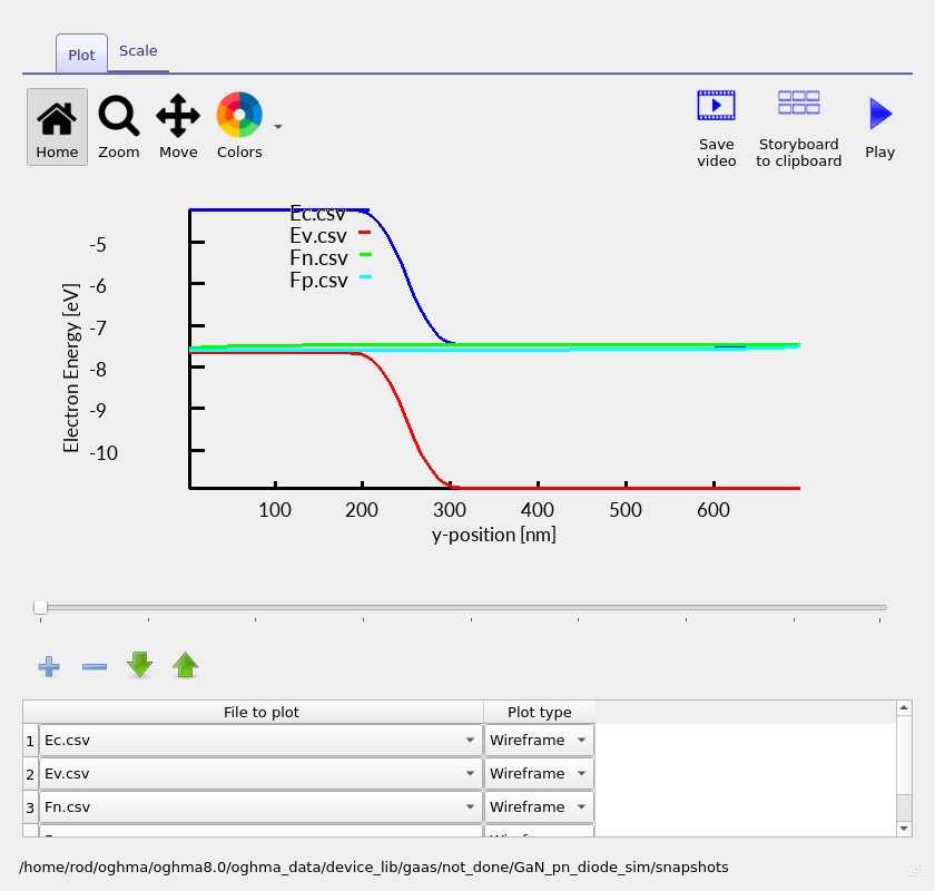
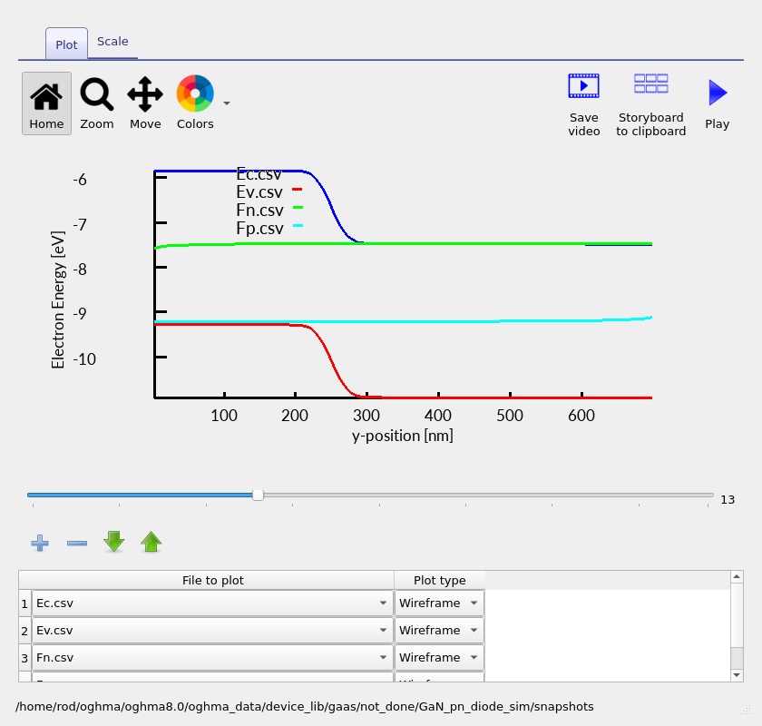
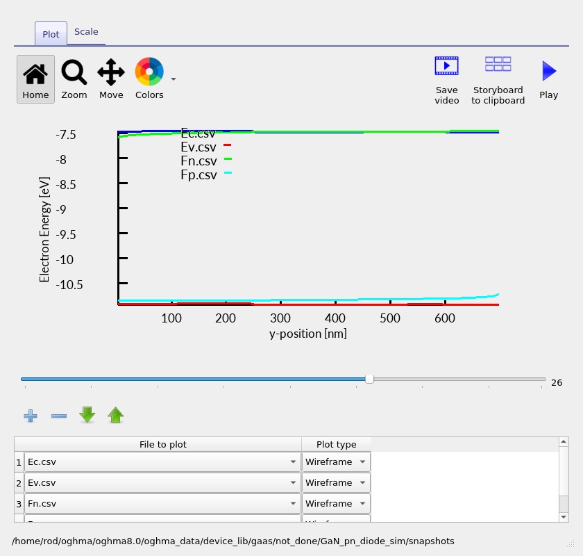
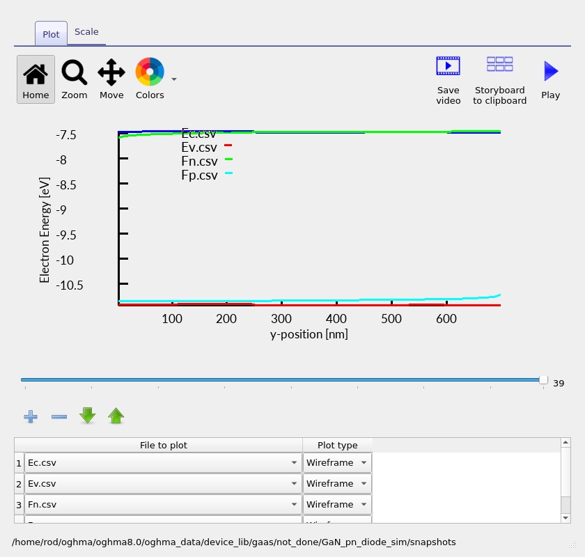
In a GaN homojunction, both sides use the same semiconductor, so the band-edge variation across the PN boundary is predominantly due to electrostatic band bending. Compare the barrier near the p–n interface at low bias with the profile after forward injection has increased. The n/n⁺ donor step can affect local bending without changing the fundamental GaN bandgap.
6.2 Electron and hole carrier densities
The saved free-electron and free-hole density profiles (Q_nfree.csv and Q_pfree.csv) provide a direct picture of majority and minority carriers. In the first snapshot, electrons dominate on the n-type side and holes dominate on the p-type side, with strong changes near the depletion region. Under forward bias, minority-carrier injection raises the carrier populations on both sides of the junction, eventually changing the spatial shape of the density profiles.
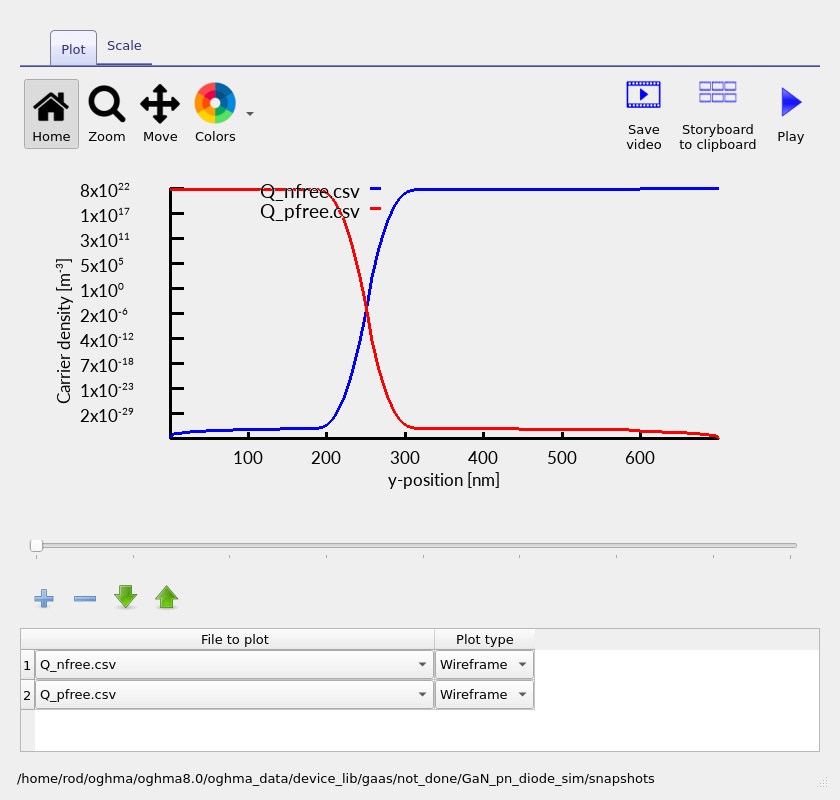
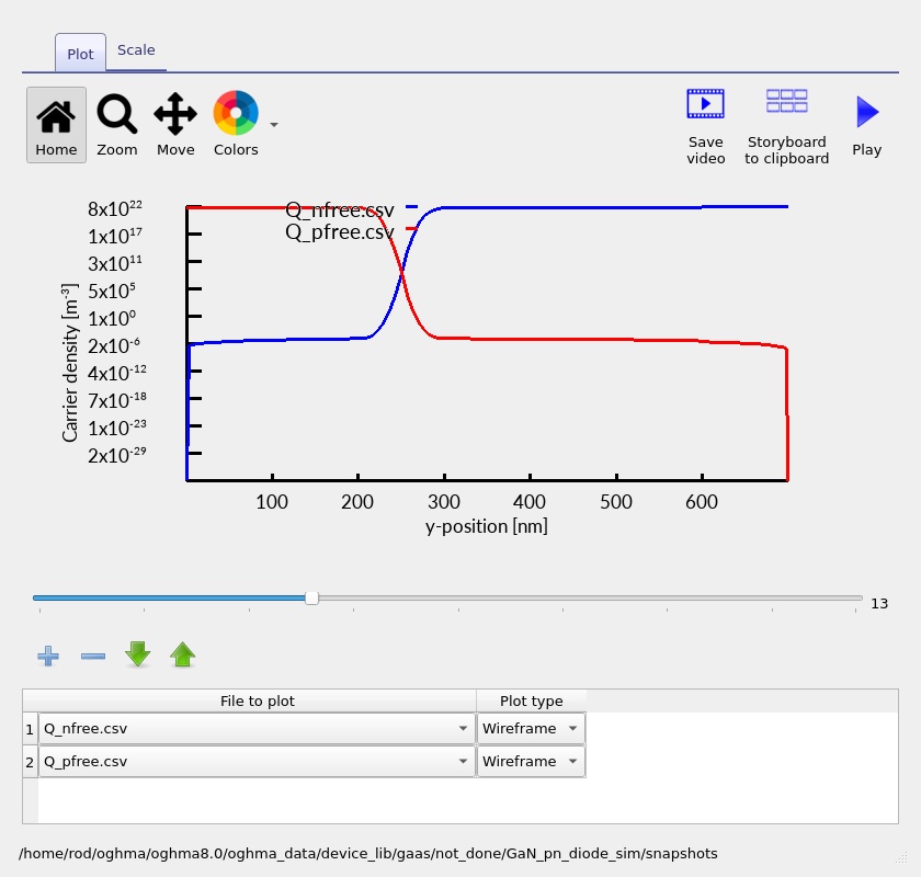
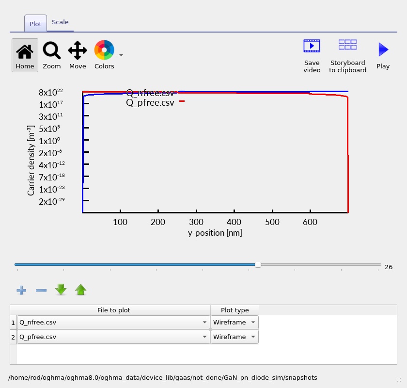
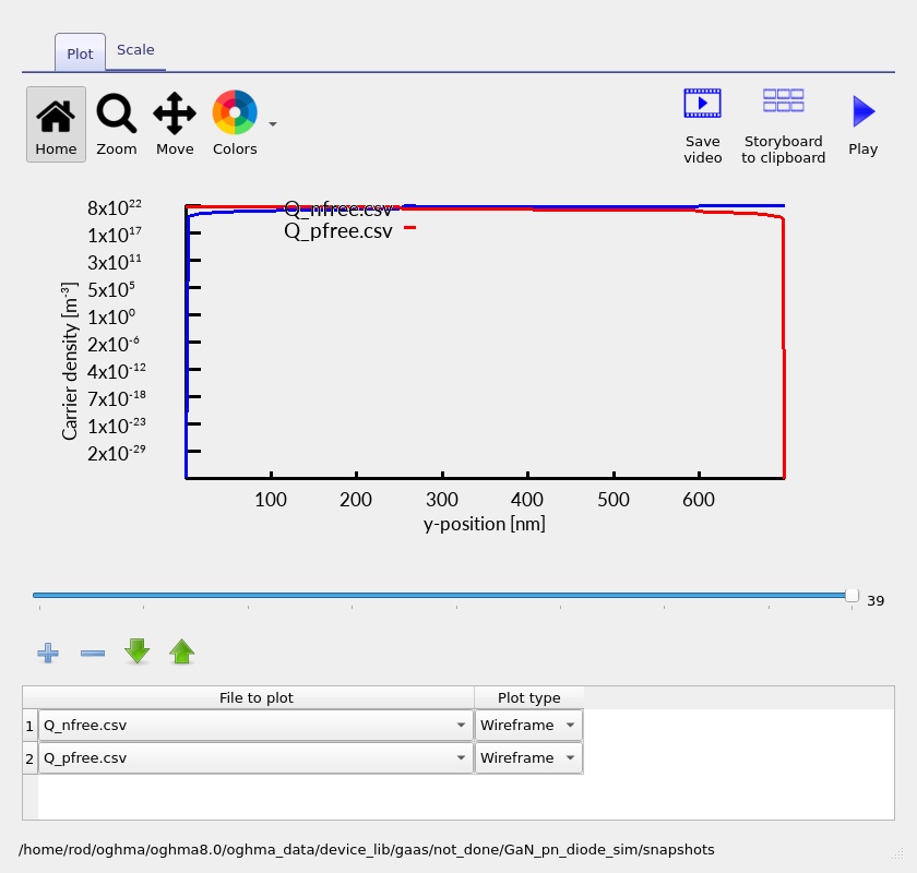
The logarithmic density scale is particularly helpful when comparing minority and majority carriers, which may differ by many orders of magnitude. Do not equate the nominal Mg acceptor concentration with the free-hole concentration without considering acceptor ionisation; incomplete Mg activation is an important feature of experimental p-GaN.
6.3 Electron and hole current densities
Plot Jn.csv and Jp.csv to examine the division of current between electrons and holes. In steady state, the electron and hole currents can exchange weight along the device as carriers recombine. Subject to sign conventions, their total electrical current should be approximately position independent when there is no net accumulation of charge.
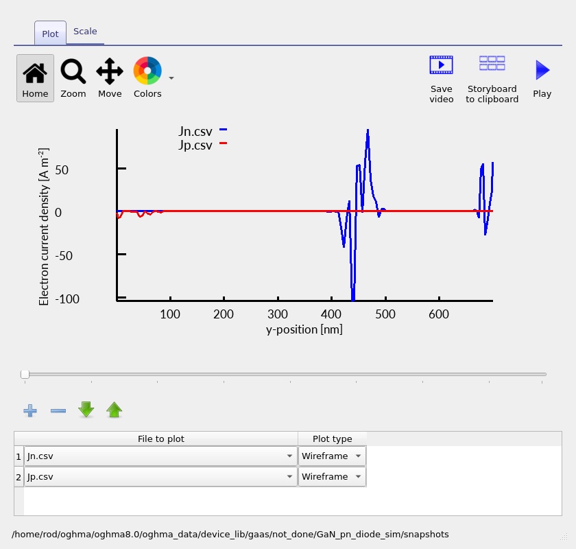
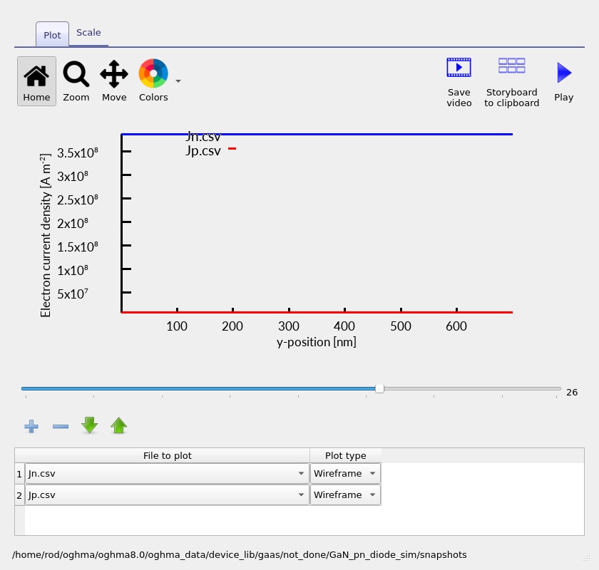
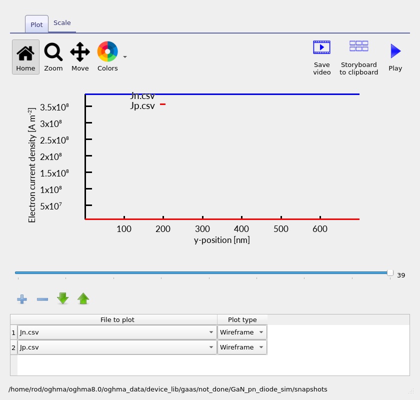
The low-current screenshot contains sharp numerical features. Such structure can arise when small current components are evaluated from opposing drift and diffusion fluxes or when a steep transition is under-resolved. It should not automatically be interpreted as a physical current spike. Evaluate solver convergence and compare the total current through the device before making a quantitative claim.
6.4 Recombination mechanisms
The recombination snapshots combine free-to-free and SRH-related rates (R_nfree_to_pfree.csv and R_ss_srh.csv in the saved screenshot sequence). At low injection, defect-mediated recombination may be concentrated around the junction, where both carrier types are available; at stronger forward bias, the spatial distribution of recombination broadens as minority-carrier populations rise. The extent and relative size of these channels depend on the numerical material parameters and must not be inferred from a peak height alone.
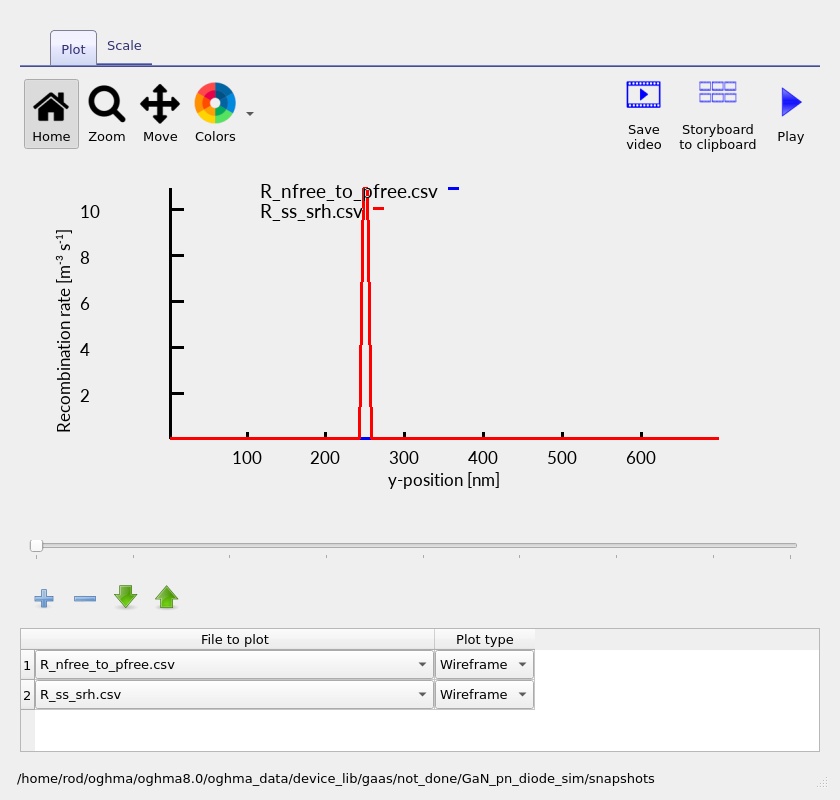
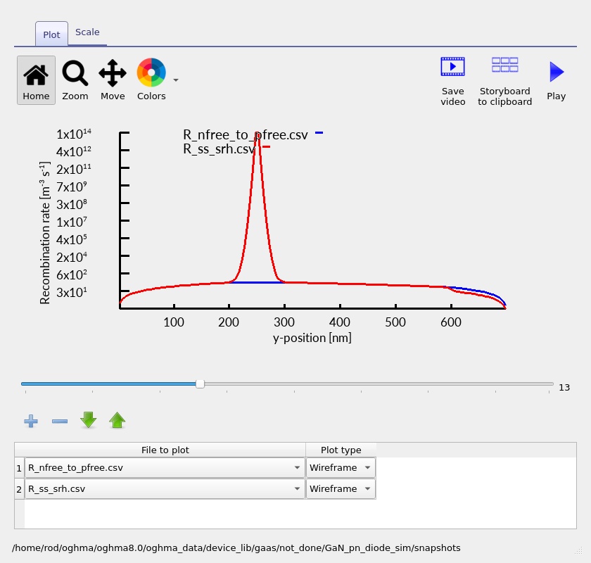
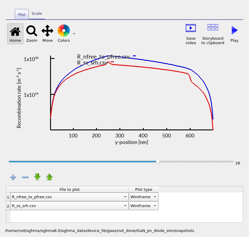
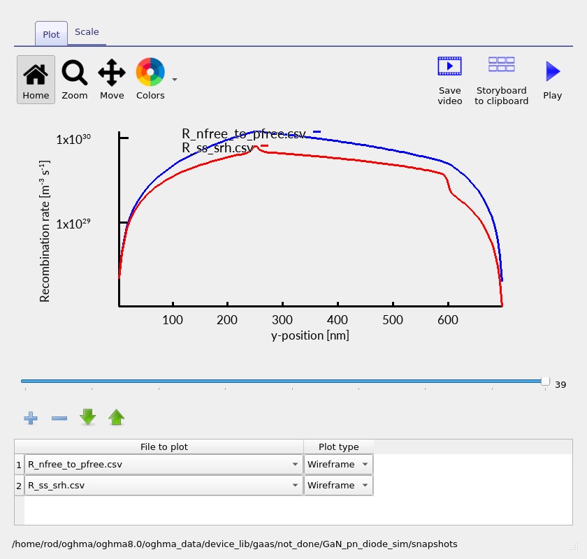
Comparing the recombination profiles at different forward biases reveals where injected electrons and holes interact most strongly. This spatial information complements the J–V curve and helps connect changes in current to the carrier populations inside the junction.
6.5 Electron and hole rate profiles
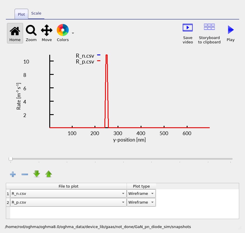
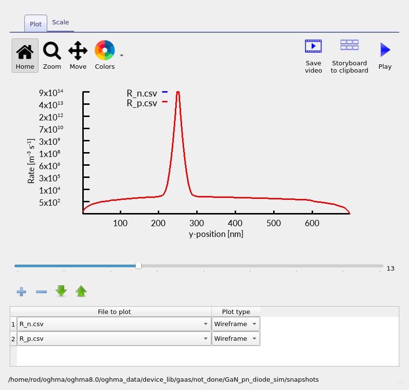
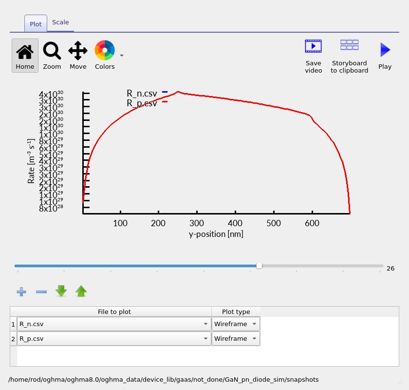
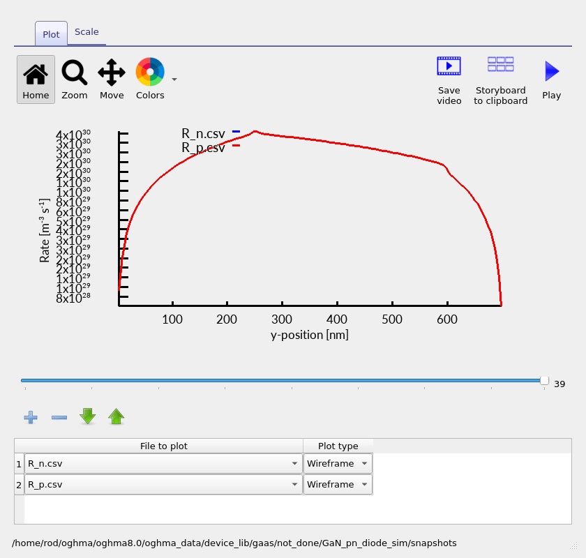
The electron and hole rate outputs (R_n.csv and R_p.csv) provide a further diagnostic of local carrier balance. Their signs and individual components should be interpreted according to OghmaNano's output convention. Compare the sharp low-bias features with the broader distributions under stronger injection; physical interpretation should focus on the consistent trends, not on interpreting each narrow numerical excursion as a separate mechanism.
7. Exercises and interpretation
8. Modelling assumptions and further analysis
The simulation uses a 1D, steady-state drift–diffusion model of a compact 700 nm GaN semiconductor stack, with ohmic boundary conditions at the contacts. This formulation is particularly useful for investigating how junction doping, material parameters and recombination affect the internal band structure and J–V response. Studies of complete power-device layouts can build on this model by incorporating device geometry, contact resistance and thermal behaviour.
The p-GaN layer is specified by a nominal Mg acceptor density. Because Mg acceptors in GaN are relatively deep, their electrical activation and the resulting hole density require care. The details depend on the material model used for carrier statistics and doping ionisation. Likewise, interface defects, bulk traps, carrier mobilities and recombination coefficients influence the calculated electrical response.
The 0–5 V sweep provides a detailed view of forward conduction, from the onset of carrier injection to the higher-current regime. Extending the sweep into reverse bias provides another useful direction for analysing depletion and electric-field behaviour. More advanced power-device studies may additionally include high-field effects and geometry-dependent voltage blocking.
For research-level quantitative predictions, check the evaluated GaN material properties, inspect the solver residual and current continuity, refine the spatial mesh, and compare with experimental measurements or literature data for a closely matched structure. These checks help extend the introductory model towards quantitative comparison with fabricated devices.
9. Next steps
Having completed the baseline J–V sweep, the next useful investigation is to vary the p- and n-type doping and compare the resulting band bending and depletion-region behaviour. A complementary study is to introduce a lightly doped central region and compare the GaN PN and PIN architectures. Those changes demonstrate how layer design affects electrostatics, forward injection and the potential for reverse-voltage support.