

InP PN Junction Diode Simulation: Drift–Diffusion, Rectification and Carrier Recombination
1. Introduction: an InP rectifying junction
Indium phosphide (InP) is a direct-bandgap III–V semiconductor used as a foundation for high-speed electronic devices and integrated photonic technologies. A PN junction diode is one of its simplest and most instructive device structures: a p-type region meets an n-type region, creating a built-in electric field and a potential barrier that controls the movement of electrons and holes. The diode conducts strongly under forward bias and suppresses carrier injection under reverse bias, producing electrical rectification.
InP has a room-temperature bandgap of approximately 1.34 eV and a comparatively high electron mobility. These properties make InP junction transport relevant to compound-semiconductor electronics and to understanding the semiconductor interfaces used in InP-based device platforms. The example in this tutorial demonstrates the electrical operation of a compact p-InP/n-InP homojunction with an n⁺ contact-side layer.
Rather than fitting the J–V curve to an ideal-diode equation alone, OghmaNano solves the coupled Poisson and drift–diffusion continuity equations. The resulting data reveal both the terminal current and the internal distribution of conduction and valence band energies, electron and hole densities, quasi-Fermi levels and recombination. This enables us to explain why the diode rectifies, rather than simply observing that it does.
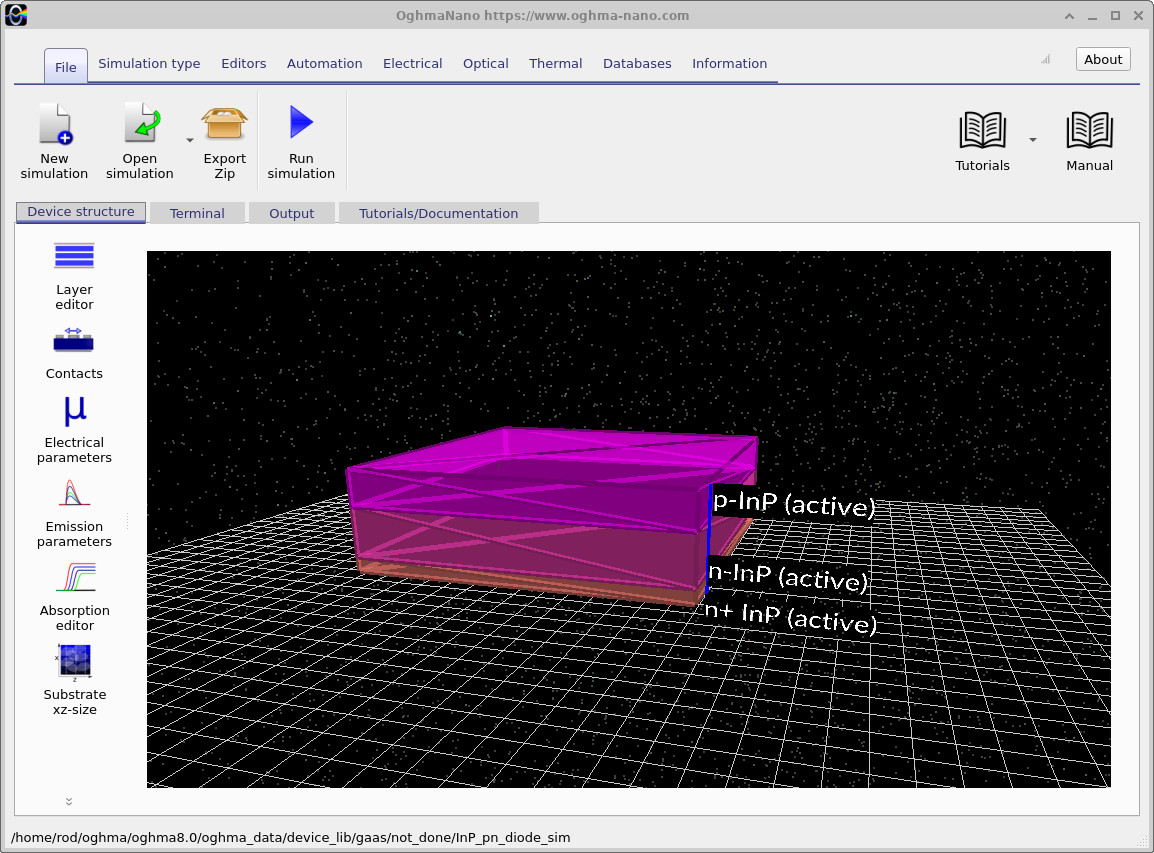
The main simulation window, shown in ??, displays the vertically layered InP device. Although the geometry is displayed in three dimensions, the electrical problem solved here is one-dimensional along the growth direction.
2. Making a new simulation
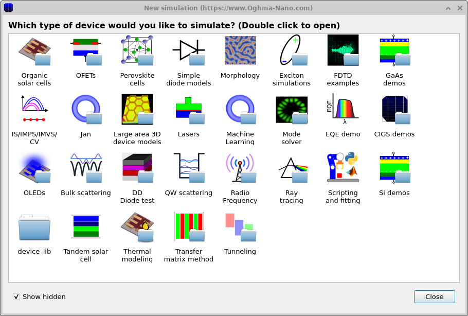
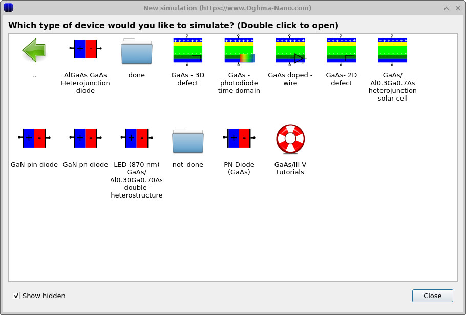
In the OghmaNano main window, select New simulation. The simulation chooser opens with the available example categories (??). Open the III–V/InP demonstrations and choose the InP PN diode example (??). The precise position of the example may vary between OghmaNano versions.
After the example opens, select the Device structure tab and open the Layer editor. Check the layer names, their thicknesses and the associated electrical material models before running the simulation. The following sections explain what each region contributes to the overall diode response.
3. Examining the device structure, contacts and doping
3.1 Semiconductor layer structure
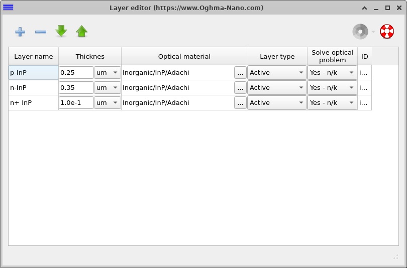
The electrical device contains three InP layers with a total semiconductor thickness of 700 nm. The p-InP and n-InP layers form the rectifying homojunction, while the n⁺-InP region provides a more heavily doped cathode-side region. The layer assignments are visible in the editor (??).
| Layer | Thickness | Nominal doping | Role |
|---|---|---|---|
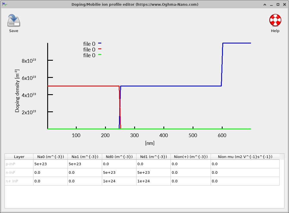
| p-InP | 250 nm | \(N_A=5\times10^{17}\,\mathrm{cm^{-3}}\) | Hole-majority region and anode side |
| n-InP | 350 nm | \(N_D=5\times10^{17}\,\mathrm{cm^{-3}}\) | Electron-majority region forming the junction |
| n⁺-InP | 100 nm | \(N_D=1\times10^{18}\,\mathrm{cm^{-3}}\) | More heavily doped cathode-side layer |
The 200 nm air region shown in the structure editor is part of the display and surrounding optical geometry, rather than the semiconductor electrical stack. Its thickness is therefore excluded from the 700 nm electrical-device thickness.
3.2 Doping and built-in electrostatics
Open Electrical → Doping / Ions to view the donor and acceptor concentrations (??). The net doping changes sign at the interface between p-InP and n-InP, approximately 250 nm from the top of the electrically active semiconductor stack. The second change, between n-InP and n⁺-InP, modifies the electron density towards the cathode but does not create another PN junction.
At equilibrium, electrons tend to diffuse from the n-type region into the p-type region, while holes diffuse in the opposite direction. The uncovered ionised dopants generate a field that opposes further diffusion. The resulting depletion region and internal potential barrier form the basis of the rectifying response.
\[ \frac{d}{dy}\left(\varepsilon\frac{d\phi}{dy}\right)=-\rho(y), \qquad \rho(y)=q\,[p-n+N_D^+-N_A^-]. \]Here \(\phi\) is the electrostatic potential, \(\varepsilon\) the dielectric permittivity and \(\rho\) the local charge density. The ionised dopants and mobile carriers determine the local electric field, while the applied voltage changes the effective barrier for carrier injection.
3.3 Electrical contacts
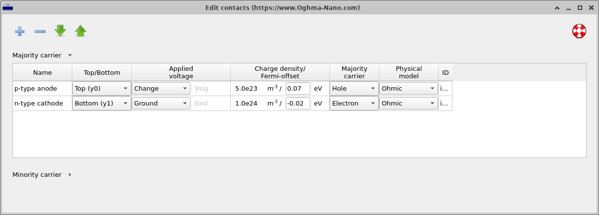
The model uses a hole-majority ohmic boundary at the anode and an electron-majority ohmic boundary at the cathode. These boundary conditions are appropriate for studying the junction response without introducing an additional injection barrier at the contacts. In fabricated devices, the contact metallisation and processing determine how closely the contacts approach ideal ohmic behaviour.
4. Material models and transport parameters
4.1 Lua material models: where the InP parameters come from
One of the important features of this InP diode example is that the electrical material parameters are defined using Lua material models. This gives a clear connection between a semiconductor's physical properties and the drift–diffusion solution. The p-InP, n-InP and n⁺-InP regions all reference the same material definition, Inorganic/InP/InP.lua. Their different electrical behaviour follows primarily from the doping profile, rather than from assigning three unrelated sets of material constants.
To examine the model, open Device structure → Electrical parameters (the electrical material editor) and select one of the InP layers. The Code editor tab displays the Lua material script associated with that region; the Parameters tab displays its evaluated material properties. These two views should be used together. The code defines how the properties are obtained, while the evaluated values reveal what the electrical solver actually receives.
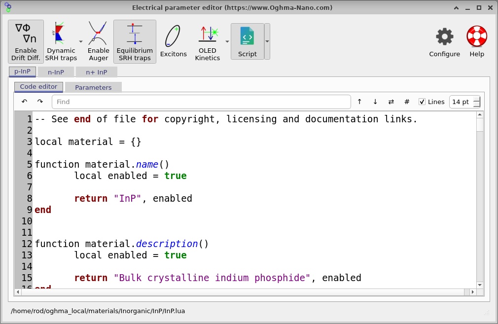
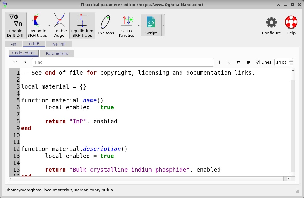
Inorganic/InP/InP.lua.The images in ?? and ?? show how the code editor is accessed. The simulation's layer configuration is the authority for the assigned material model: every active region in this example is associated with the InP Lua file. The image filenames are inherited from the screenshot-capture sequence and do not determine which semiconductor is simulated.
In the supplied simulation, the db_overrides switches are set to false for the key transport and band parameters. OghmaNano is therefore configured to obtain the corresponding values from the material database/Lua model instead of forcing the fallback numbers recorded elsewhere in the JSON. This matters when inspecting the configuration: the effective values shown in the Parameters tab are more informative than the stored defaults in an inactive override field.
4.2 Band structure, density of states and mobility
The first quantities to check in the evaluated Parameters tab are the bandgap \(E_g\) and electron affinity \(\chi\). The bandgap sets the separation between the conduction and valence bands, while electron affinity locates the conduction-band edge relative to a vacuum-energy reference. For InP, the room-temperature bandgap is approximately \(1.34\,\mathrm{eV}\). A useful initial consistency check is whether the separation of \(E_c\) and \(E_v\) in the resulting band diagram agrees with the evaluated bandgap.
The effective conduction- and valence-band densities of states, \(N_c\) and \(N_v\), influence the relationship between carrier concentration and quasi-Fermi-level position. They therefore contribute to the equilibrium electron and hole populations and to the injection response under forward bias. The relative permittivity \(\varepsilon_r\) enters Poisson's equation and influences the electrostatic potential and depletion width. These quantities should be inspected as a consistent set, not as independent numerical tuning parameters.
The electron and hole mobilities, \(\mu_n\) and \(\mu_p\), determine the carrier drift response to an electric field; diffusion additionally depends on carrier-density gradients. In the one-dimensional model the current densities are written as
\[ J_n=q\mu_n nE+qD_n\frac{dn}{dy},\qquad J_p=q\mu_p pE-qD_p\frac{dp}{dy}. \]Here \(n\) and \(p\) are the local electron and hole densities, \(E\) is the electrical field, and \(D_n\), \(D_p\) are diffusion coefficients. The two current components can vary considerably through the diode even when the total steady-state current is approximately position-independent. This is why later sections examine \(J_n\) and \(J_p\) alongside the carrier-density profiles.
4.3 How to inspect and compare the material settings
In the electrical editor, select p-InP and examine its Lua code and evaluated parameters. Then switch to n-InP, and finally to n⁺-InP. Compare the assigned material model, bandgap, electron affinity, mobilities, effective densities of states, permittivity and recombination coefficients. For this homojunction, the same underlying InP model is used in all three regions; the main deliberate change between regions is their acceptor or donor concentration.
It is worth separating two ideas: the material model describes properties of InP, whereas the doping profile establishes which charge carriers dominate locally and where the junction lies. This distinction becomes especially useful when moving from a PN homojunction to an InP-based heterojunction, where differences between material models can themselves produce band offsets. In this diode, the conduction- and valence-band bending seen in the snapshots primarily reflects electrostatics across the p/n transition.
For a reproducible study, keep the Lua material model fixed when changing the doping concentrations. Conversely, if investigating the sensitivity of the result to a mobility or recombination coefficient, change that material parameter deliberately and compare the resulting J–V curve, carrier densities and internal current profiles. The parameter editor and Lua code views provide the link between the physical input assumptions and the simulated output.
4.4 Recombination parameters
The InP regions include Shockley–Read–Hall (SRH) recombination and a free-carrier recombination channel through the evaluated material model. SRH recombination describes defect-assisted capture of electrons and holes; free-to-free recombination is particularly relevant in direct-bandgap InP because electron–hole transitions can occur radiatively. In the present exercise, both are useful as carrier-loss processes that modify the electrical current.
\[ R_{\mathrm{rad}}=B\left(np-n_i^2\right), \qquad R_{\mathrm{SRH}}=\frac{np-n_i^2}{\tau_p(n+n_1)+\tau_n(p+p_1)}. \]The coefficient \(B\), trap lifetimes \(\tau_n\) and \(\tau_p\), and auxiliary densities \(n_1\), \(p_1\) determine the magnitude of each process. The key diagnostic in this tutorial is how the spatial distribution of recombination changes as bias drives more electrons and holes into the same region.
4.5 Mesh and numerical solution
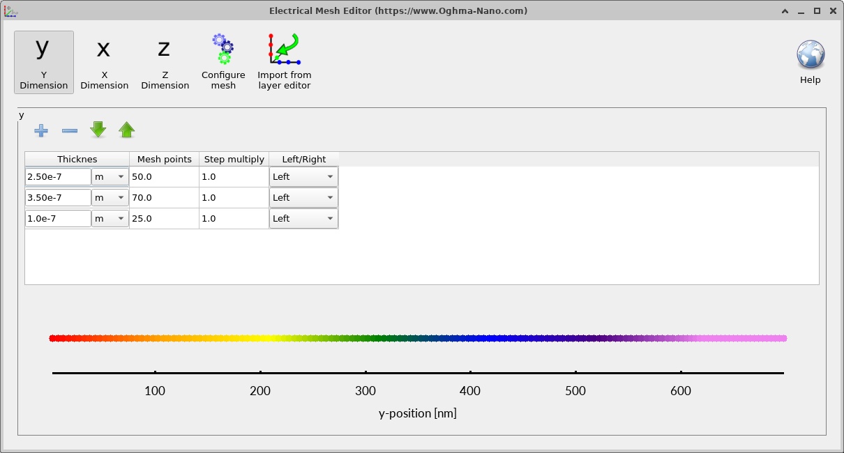
The electrical calculation uses a one-dimensional mesh of 150 points across 700 nm, corresponding to an average spacing of roughly 4.7 nm. The coupled nonlinear equations are solved using Newton iteration and the UMFPACK sparse linear solver. This mesh is a useful starting point for examining the junction and the quasi-neutral regions.
The output includes convergence information and bias-dependent device profiles. A good first check is to look for a smooth J–V curve and then confirm that the electron and hole currents obey overall steady-state current conservation. The mesh editor is shown in ??.
5. Running the simulation and interpreting the J–V response
Return to the main window and select Run simulation. OghmaNano sweeps the applied voltage and writes the converged solution at each point. The saved example file uses a 0–3 V sweep with 25 mV steps. The terminal records solver progress during the sweep, while the Output tab provides access to the resulting data.
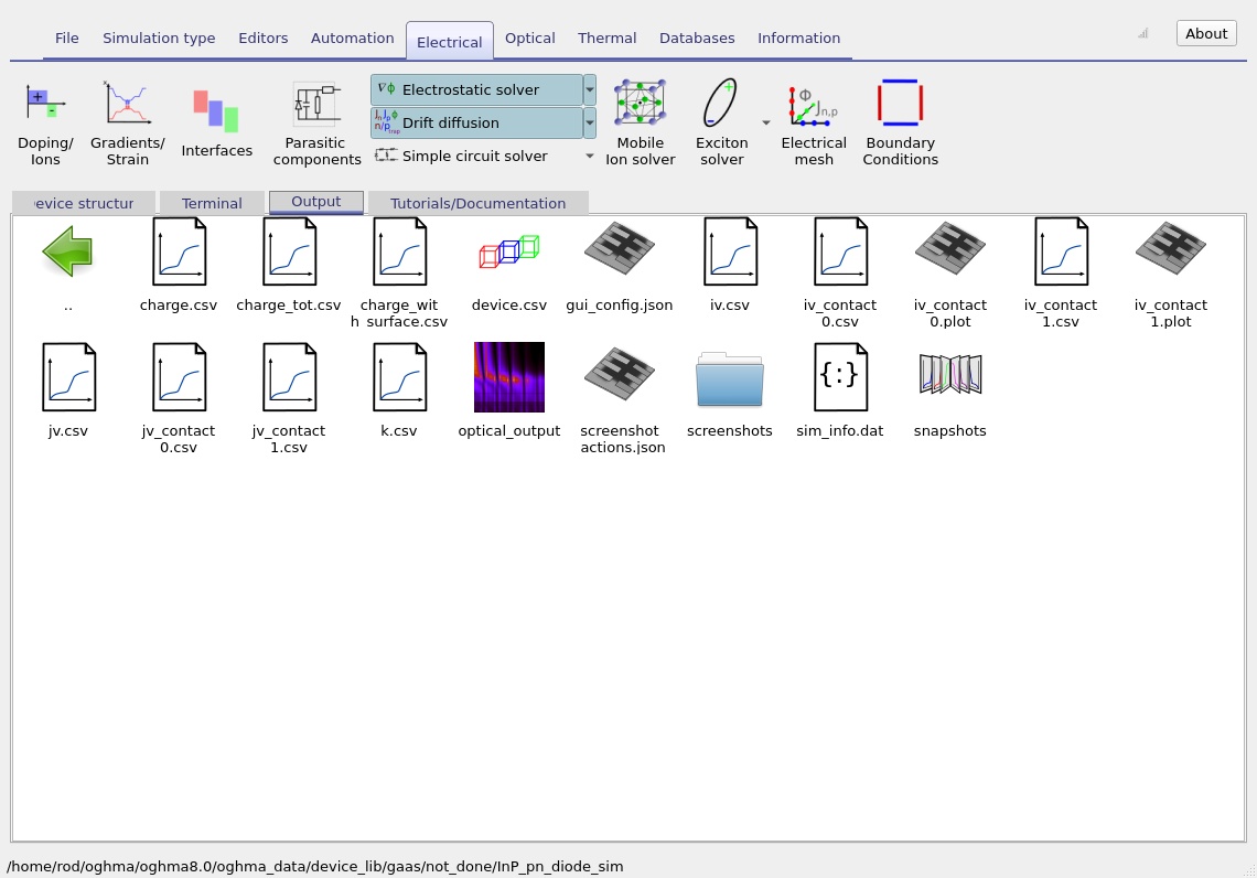
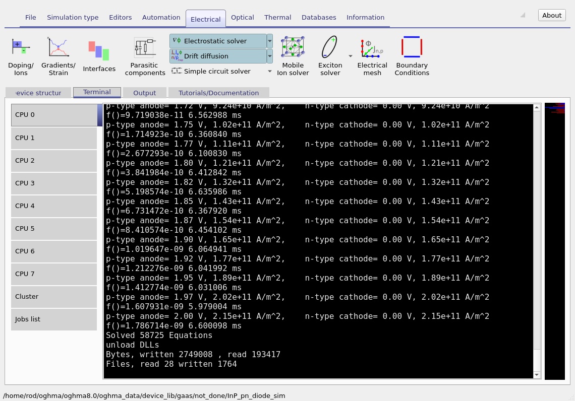
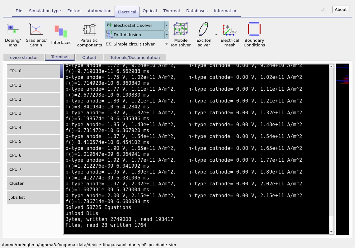
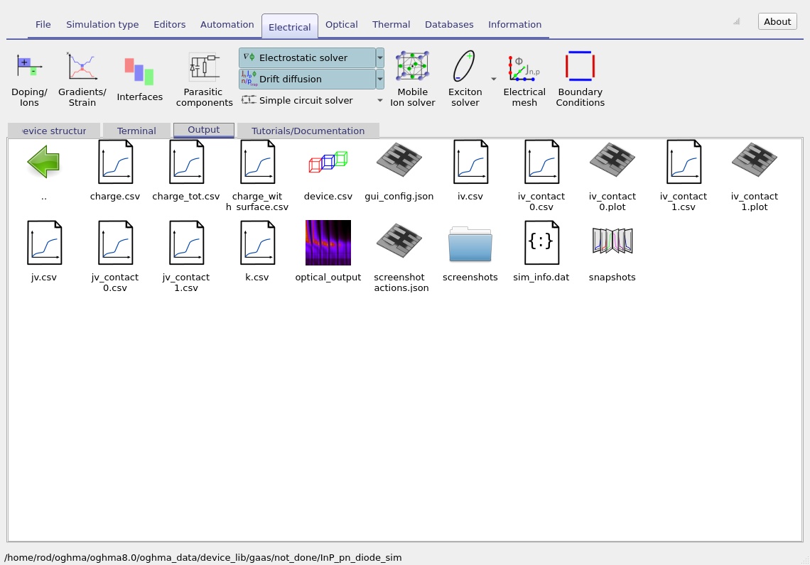
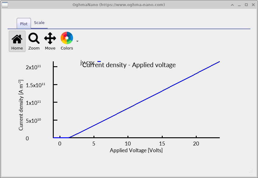
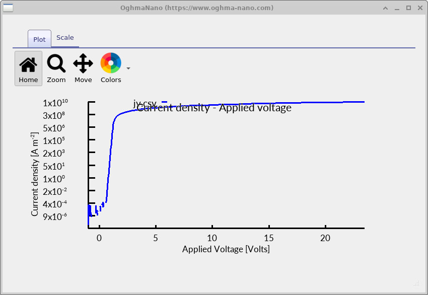
When the run has finished, the results become available in the Output tab (??). Open jv.csv to plot current density versus applied voltage. The screenshots include both a linear J–V view (??) and a logarithmic-current view (??).
5.1 Understanding the characteristic
At low applied voltage, the built-in junction barrier strongly restricts carrier injection. Increasing forward bias reduces that barrier, so electrons and holes enter the opposite side more readily and the total current rises. In the intermediate regime, the current is often approximately exponential with voltage; at larger currents, transport and resistive losses can modify the slope.
\[ J\approx J_0\left[\exp\!\left(\frac{qV}{nk_{\mathrm B}T}\right)-1\right]. \]This ideal-diode expression provides a useful reference for analysing an approximately exponential interval, but it is not imposed by the drift–diffusion model. The ideality factor \(n\) and prefactor \(J_0\) should be extracted only over a suitable bias interval; they can change with recombination, series resistance and contact behaviour.
The logarithmic plot helps identify the onset of appreciable current and changes in slope. The linear plot makes the magnitude and high-current shape easier to interpret. For the clearest picture of diode operation, examine both plots together with the internal band and carrier-density profiles.
6. Internal profiles: how the diode works
The snapshots directory contains spatial profiles saved at selected bias points during the J–V sweep. The supplied screenshots sample four positions through that sweep. They provide a progression from low injection towards stronger forward bias. The four images within each group correspond to the same selected slider positions, allowing the different physical quantities to be compared directly.
6.1 Conduction and valence bands, and quasi-Fermi levels
Open the snapshot viewer and select Ec.csv, Ev.csv, Fn.csv and Fp.csv. These are the conduction-band edge, valence-band edge, electron quasi-Fermi level and hole quasi-Fermi level. Their spatial separation and slopes reveal the potential barrier, the applied-bias response and the departure from equilibrium.
At low injection, the band edges bend across the junction as a result of the built-in electrostatic field. Under increasing forward bias, the effective barrier is reduced, and electron and hole quasi-Fermi levels separate as carriers are driven through the device. The key point is that InP remains the same semiconductor on both sides of the junction: the changing profiles reflect its doping-defined electrostatics and carrier injection.
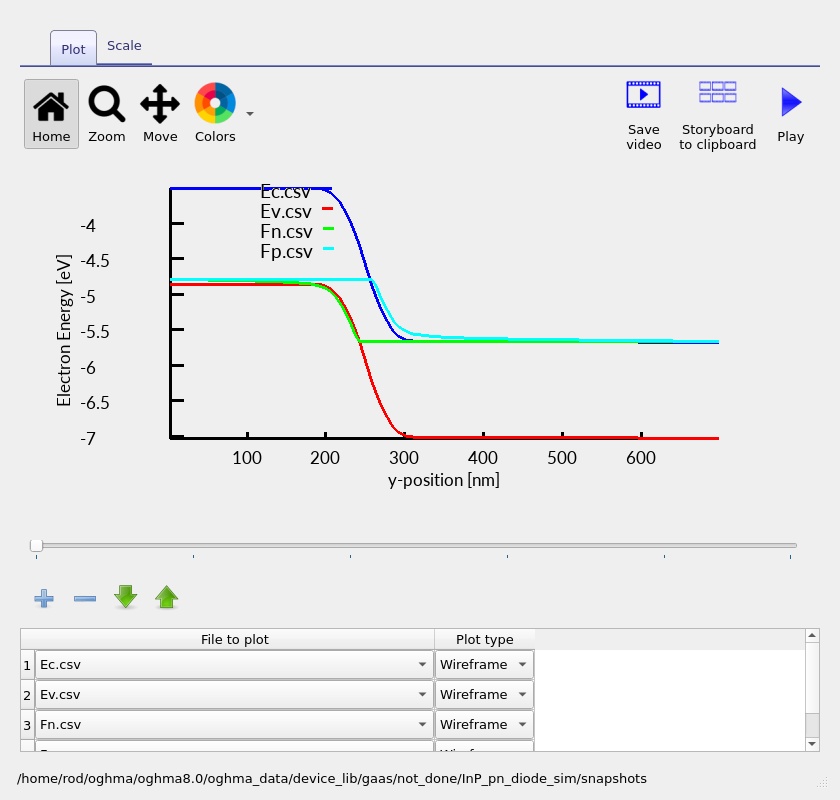
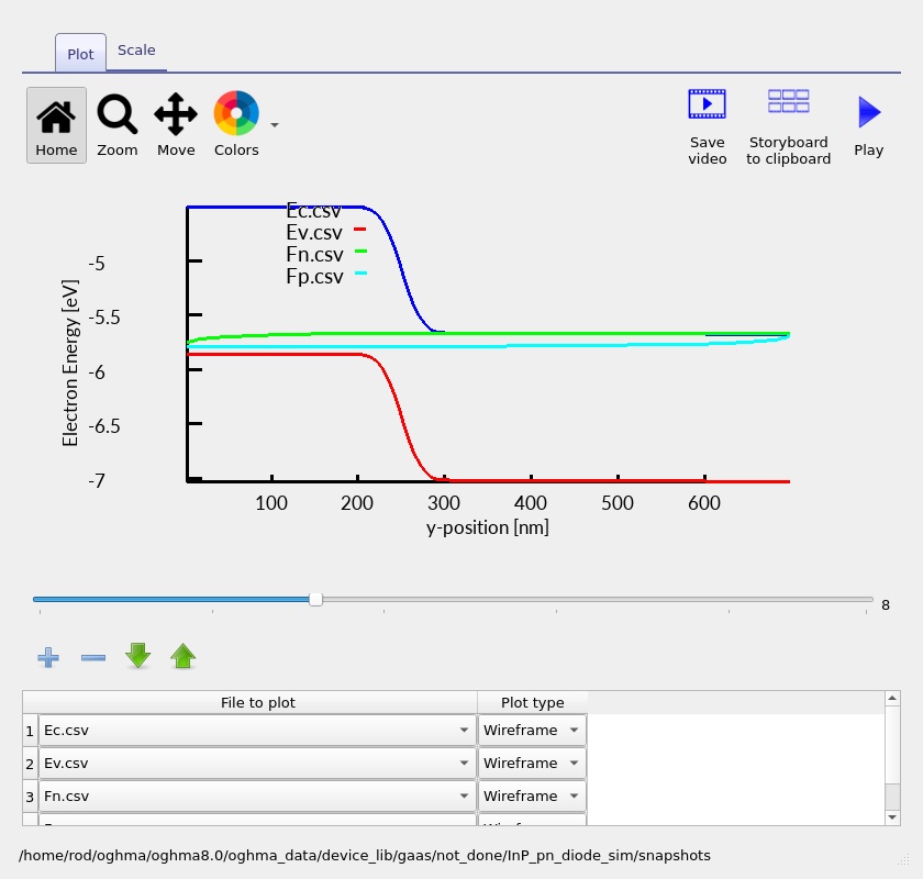
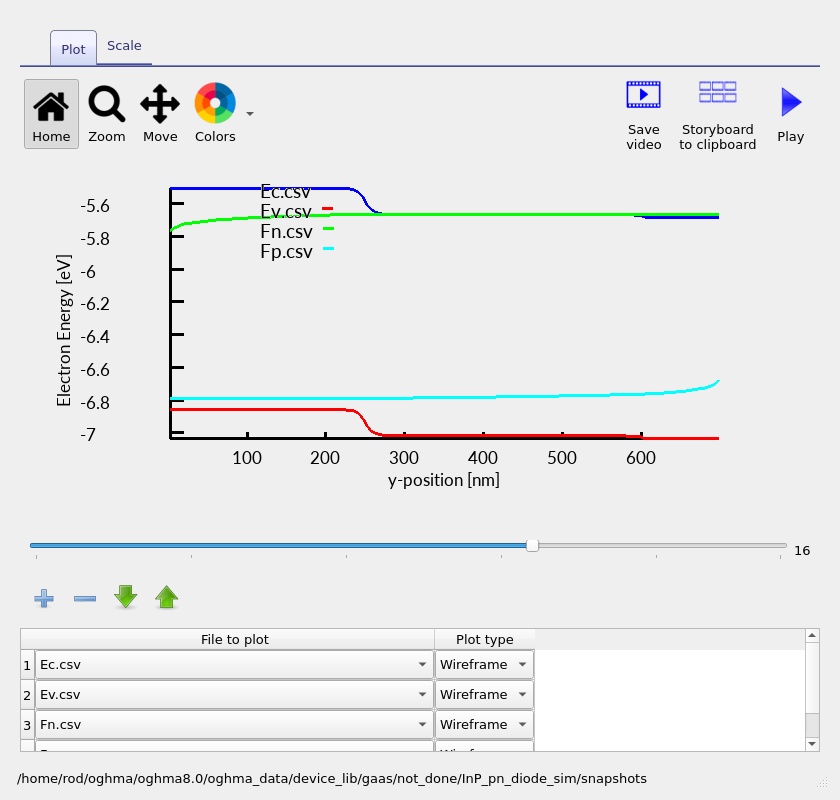
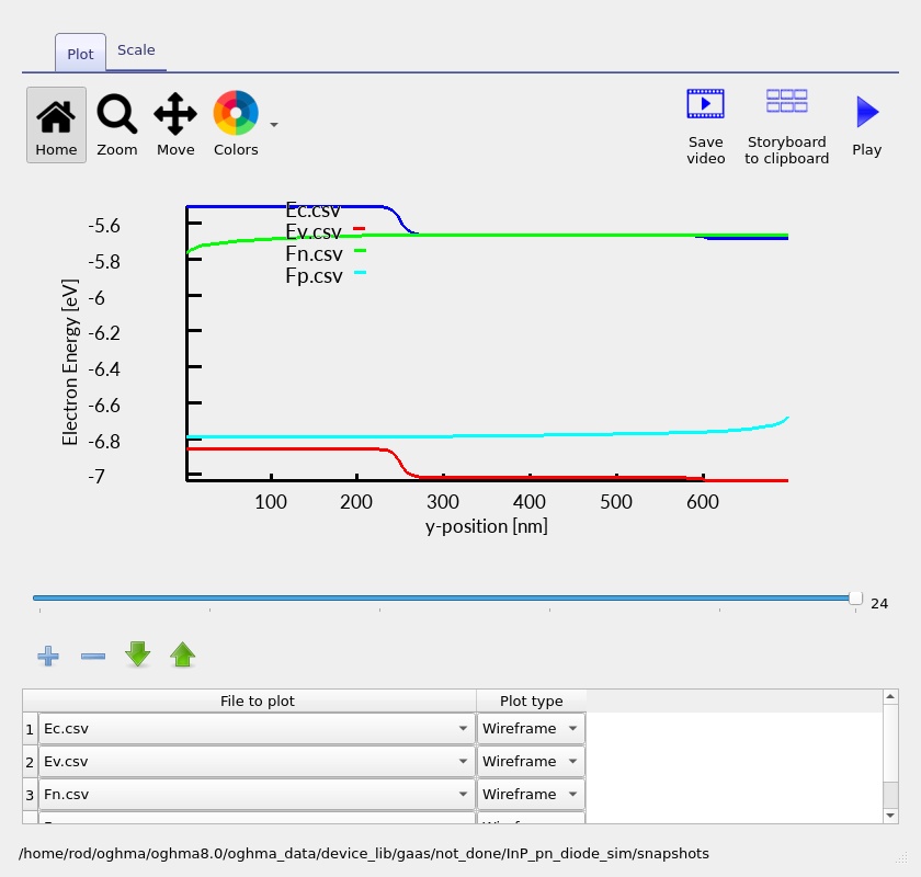
The comparison between ?? and ?? illustrates how terminal bias changes the internal band structure. In particular, the quasi-Fermi levels provide a direct diagnostic of the nonequilibrium state established during steady-state conduction.
6.2 Electron and hole densities
Next plot Q_nfree.csv and Q_pfree.csv, which show the spatial distributions of free electrons and holes. At low bias, electrons predominate on the n-type side and holes on the p-type side. Their densities become strongly reduced around the junction, reflecting the depletion region.
As forward bias increases, minority carriers are injected into the opposite sides. This increases the overlap of electron and hole populations and changes the shape of both density profiles. At larger injection levels, the free-carrier populations across the junction differ substantially from their low-bias values.
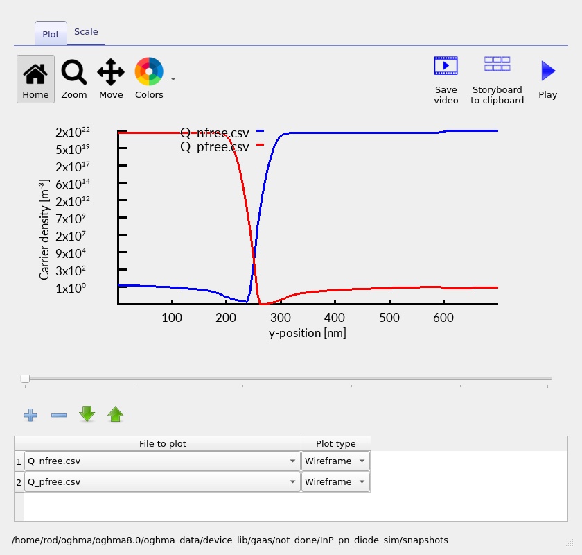
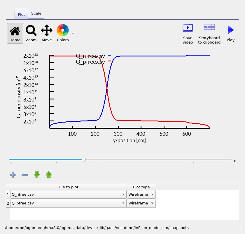
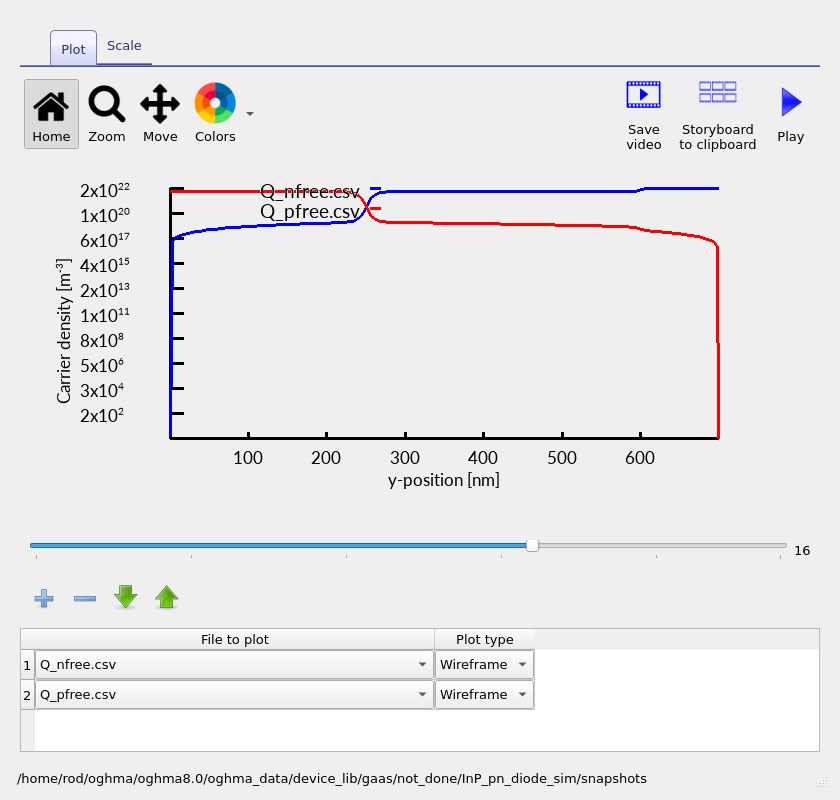
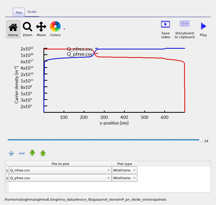
Compare the density crossover to the position of the doping transition, and then to the locations of strong band bending. This connects the contact-supplied carriers with the electrostatic barrier produced by the PN junction.
6.3 Electron and hole current densities
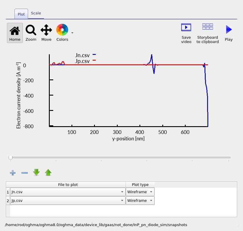
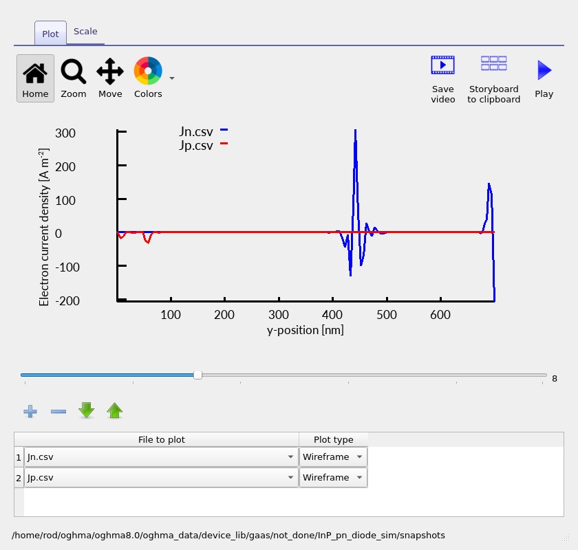
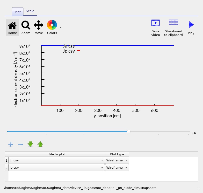
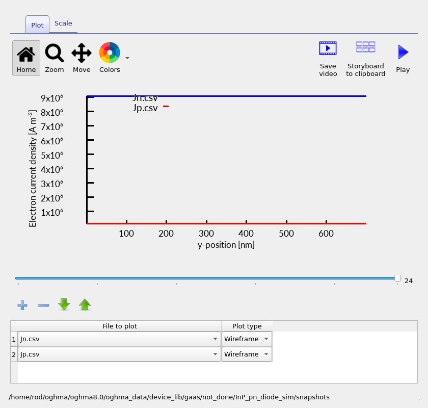
Plot Jn.csv and Jp.csv. These profiles show the electron and hole contributions to electrical current through the device. The individual components can vary with position because recombination transfers carriers between the electron and hole populations, but the total steady-state current should remain approximately constant when no net charge accumulates.
At very low current, cancellation between drift and diffusion terms can make individual current profiles appear noisy or sharply structured. The low-bias screenshots show this behaviour more strongly than the higher-current snapshots. It is useful to inspect the profiles on an appropriate scale and compare the total current with the terminal J–V value before interpreting fine numerical features.
6.4 Recombination profile
Recombination determines where injected electrons and holes are removed from their respective carrier populations. Open the snapshot viewer with R_nfree_to_pfree.csv and R_ss_srh.csv to compare the direct free-to-free and defect-assisted channels, respectively. Both processes depend on the availability of electrons and holes, so their spatial distributions evolve as the injected carrier populations change.
Near the onset of conduction, recombination can be concentrated near the junction, where electron and hole populations overlap. Under stronger forward injection the overlap spreads into a larger part of the semiconductor, and the recombination profiles can become broader. Compare the position and width of the recombination peaks with the carrier densities at the same bias.
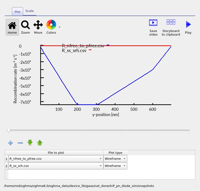
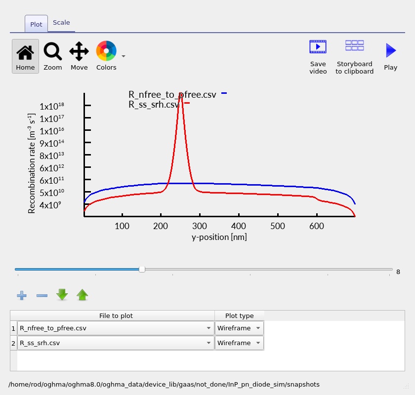
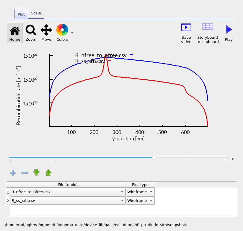
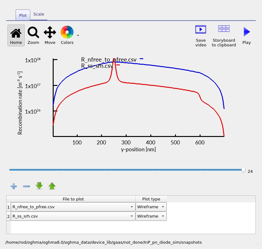
When comparing the two channels, consider both peak value and spatial integral. A sharp local peak need not dominate the integrated recombination if another channel is active over a much larger volume. This is particularly important when relating recombination profiles back to the total electrical current.
6.5 Electron and hole net rate profiles
The snapshots labelled R_n.csv and R_p.csv provide further information about the rates entering the electron and hole continuity equations. These can highlight where the balance of local generation, capture and recombination terms is most strongly concentrated. Interpret their signs according to the plotting convention used by OghmaNano.
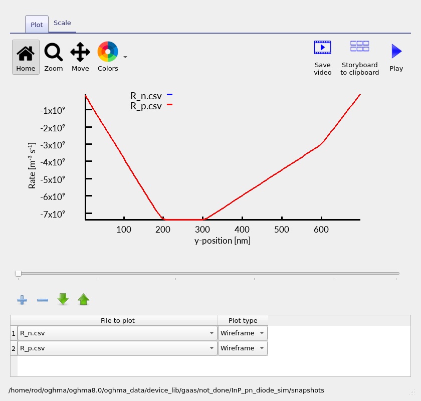
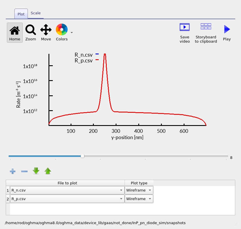
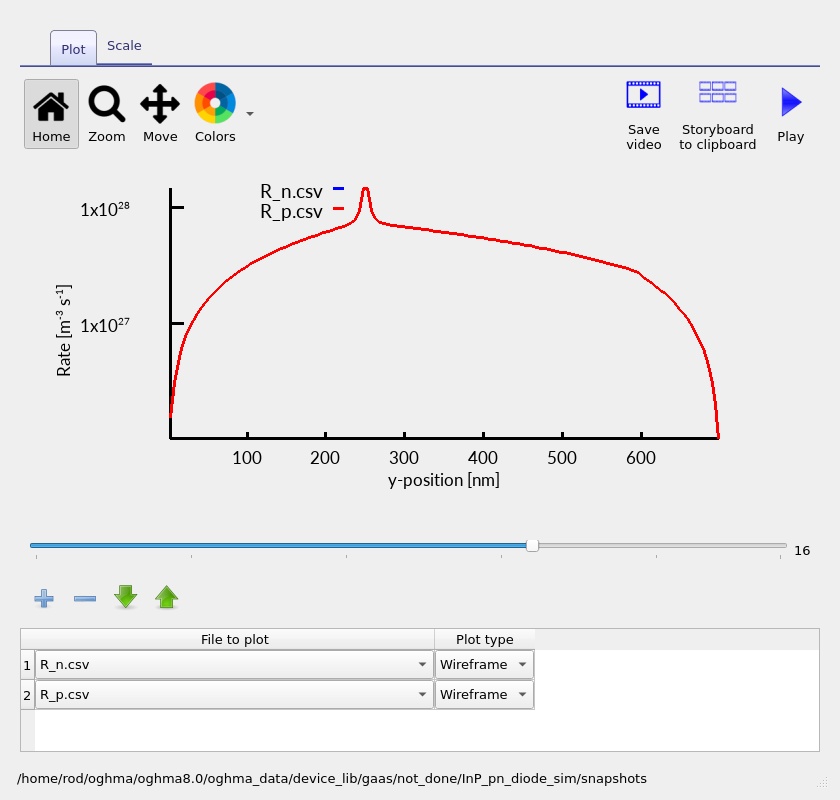
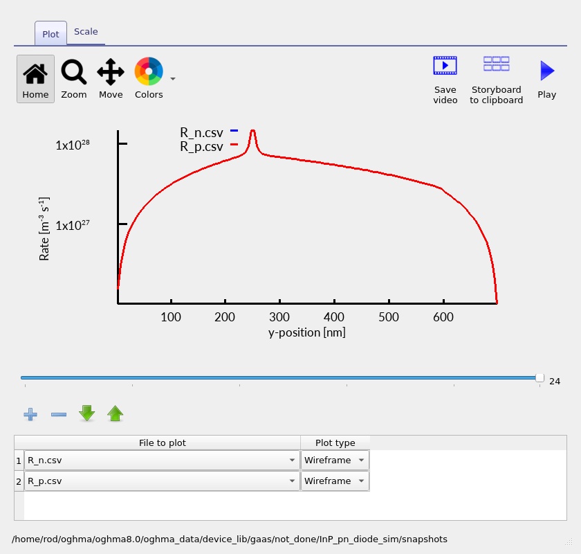
Taken together, the band structure, carrier densities, currents and rate profiles provide a complete explanation of the diode characteristic: the built-in barrier controls injection, applied bias modifies the internal electrostatics, and transport and recombination set the resulting steady-state current.
7. Exercises and interpretation
8. Model interpretation and further analysis
This example uses a one-dimensional steady-state InP drift–diffusion model, a compact p/n/n⁺ semiconductor stack and idealised ohmic terminals. It is well suited to demonstrating how electrical rectification emerges from the junction barrier and how that behaviour is connected to the spatial carrier distributions. More elaborate device studies can introduce measured contact characteristics, refined material parameters, temperature variation and additional geometric detail.
The InP material properties are obtained from the selected Lua model. For quantitative studies, confirm the evaluated bandgap, electron affinity, mobility and recombination coefficients in the material editor or output data. Check current conservation and solver residuals, and repeat representative bias points with a finer mesh to establish numerical stability.
The standard sweep in the supplied example runs from 0 to 3 V. An informative next experiment is to include a modest reverse-bias range, enabling direct comparison of forward conduction and reverse leakage. The physically relevant reverse-bias range and leakage characteristics depend on the device and on the mechanisms included in the simulation.
For further insight, vary the doping concentrations one at a time. Increasing the nominal doping generally narrows the depletion region and changes the equilibrium electrostatics; changing the recombination coefficients influences the injection-dependent current. These are useful controlled comparisons because the layer materials and geometry can remain fixed.
9. Next steps
The InP PN diode provides a useful starting point for more advanced InP-based semiconductor structures. A natural extension is to introduce a lightly doped region and compare the electrostatic and transport behaviour of a PN and PIN junction. Another direction is to examine heterostructures involving InGaAs/InP, where differences in composition introduce additional band offsets and new carrier-injection behaviour.