Optical fiber mode solver (TE/TM)
In this tutorial we calculate the guided optical modes supported by cylindrical waveguides such as optical fibers using the OghmaNano optical mode solver. Unlike slab waveguides, optical fibers confine light in two transverse dimensions, producing fully two-dimensional guided eigenmodes. The tutorial demonstrates how to build free-form optical geometries, configure the optical mesh, and visualise TE and TM modal field distributions.
1. Creating the optical fiber simulation
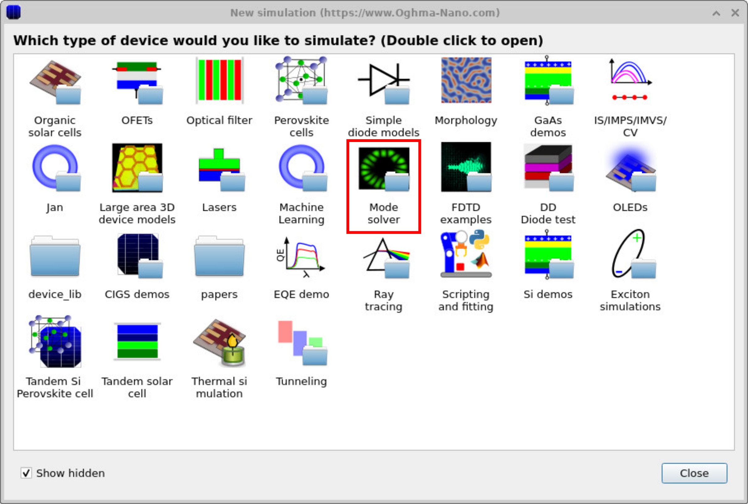
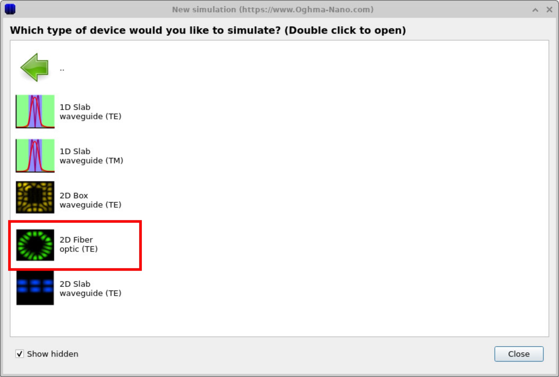
Click New simulation. This opens the library of available device categories, shown in ??. Double-click the Mode solver icon to open the optics examples folder. You’ll see a list of pre-set simulations, including 1D slab waveguides (TE/TM), 2D box guides, 2D slab guides, and a 2D fiber optic template, as shown in ??. For this tutorial, select 2D optical fiber mode solver (TE). When prompted, save the new simulation to a folder you have write access to.💡 Tip: For best performance save to a local drive such as
C:\. Simulations stored on network, USB, or cloud folders
(e.g. OneDrive) can run slowly due to heavy read/writes.
2. Building the fiber geometry
Click New simulation. This opens the library of available device categories, shown in ??. Double-click the optical mode solver icon to open the optics examples folder. You’ll see a list of pre-set simulations, including 1D slab waveguides (TE/TM), 2D box guides, 2D slab guides, and a 2D fiber optic template, as shown in ??. For this tutorial, select 2D optical fiber mode solver (TE). When prompted, save the new simulation to a folder you have write access to.
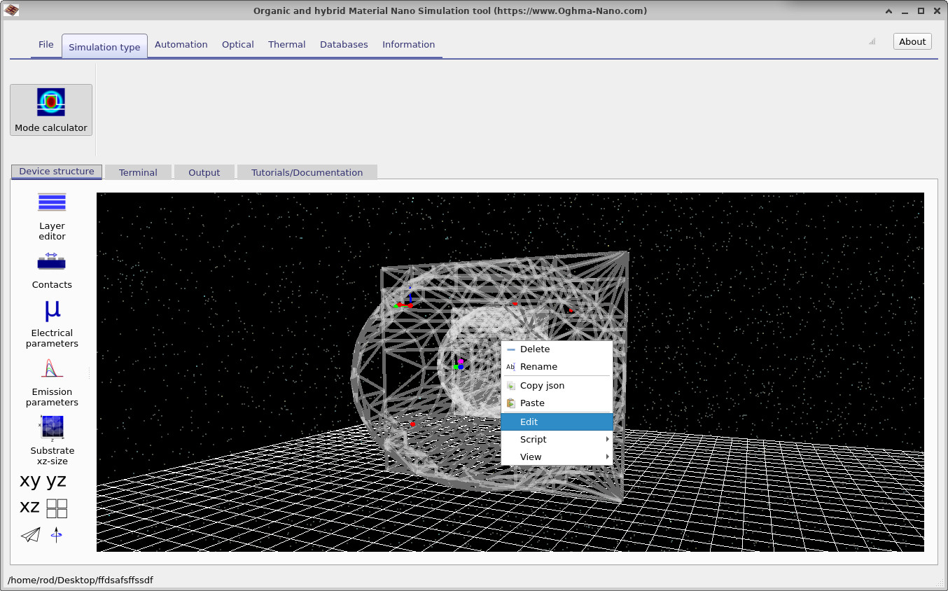
When the main simulation window opens, you will see a geometry view similar to ??. In this example, two free-form objects from the shape library have been placed inside one another to form the fiber cross-section. You can reposition objects by dragging them in the main window with the left mouse button.
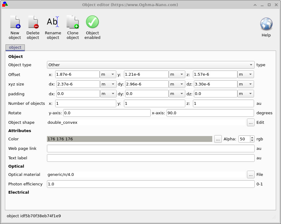
If you right-click on the inner object, a context menu appears (??). Selecting Edit opens the Object editor (??), where you can modify properties such as material, refractive index, dimensions, orientation, and position. This editor allows you to fine-tune the geometry before running the optical mode solver.
3. Running the optical mode solve
Click the Run simulation button (blue play icon) to start the calculation. Compared to the 1D slab example, this step will take longer because multiple 2D modes may exist, and each requires additional computation.
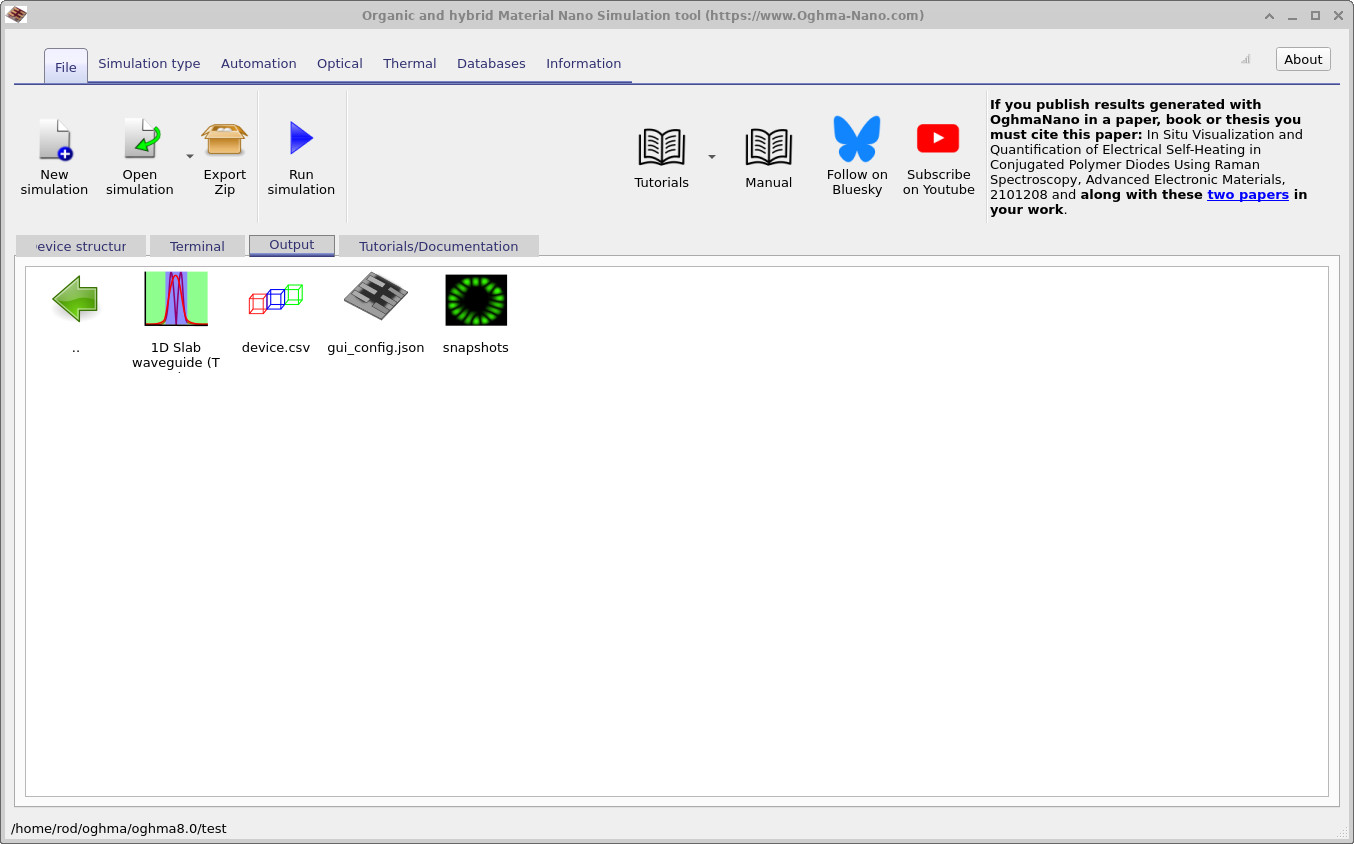
Once the run is complete, go to the Output tab of the main window
(??).
A new snapshots directory will appear containing the calculated field data.
Double-click to open it, then use the Add (+) button to load E.csv into the plot list.
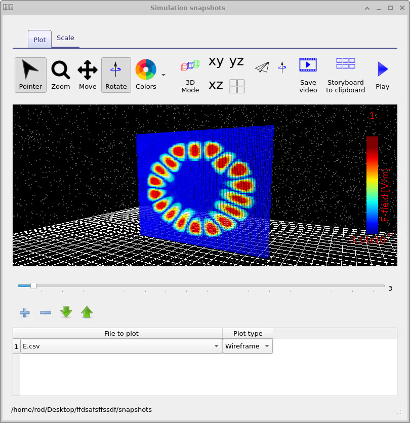
With the slider, you can step through the different optical modes that the solver has found. The Snapshots window
(??)
displays the electric field distribution for each mode.
In this fiber example, the modal profiles are slightly asymmetric because the core is not perfectly centered within the cladding.
Try adjusting the core’s position, refractive index, or radius to explore how these changes affect the supported modes.
4. Configuring the optical mesh and eigenmode search
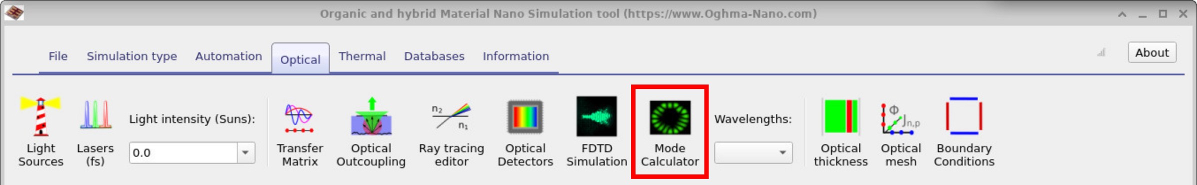
Before running the calculation, you can fine-tune the optical mesh and solver settings. The Optical ribbon provides access to the Optical mesh editor (??), where you define the grid resolution in both the X and Y directions. A sufficiently fine mesh is essential for capturing sharp field variations, especially near high-index contrasts or small structures.
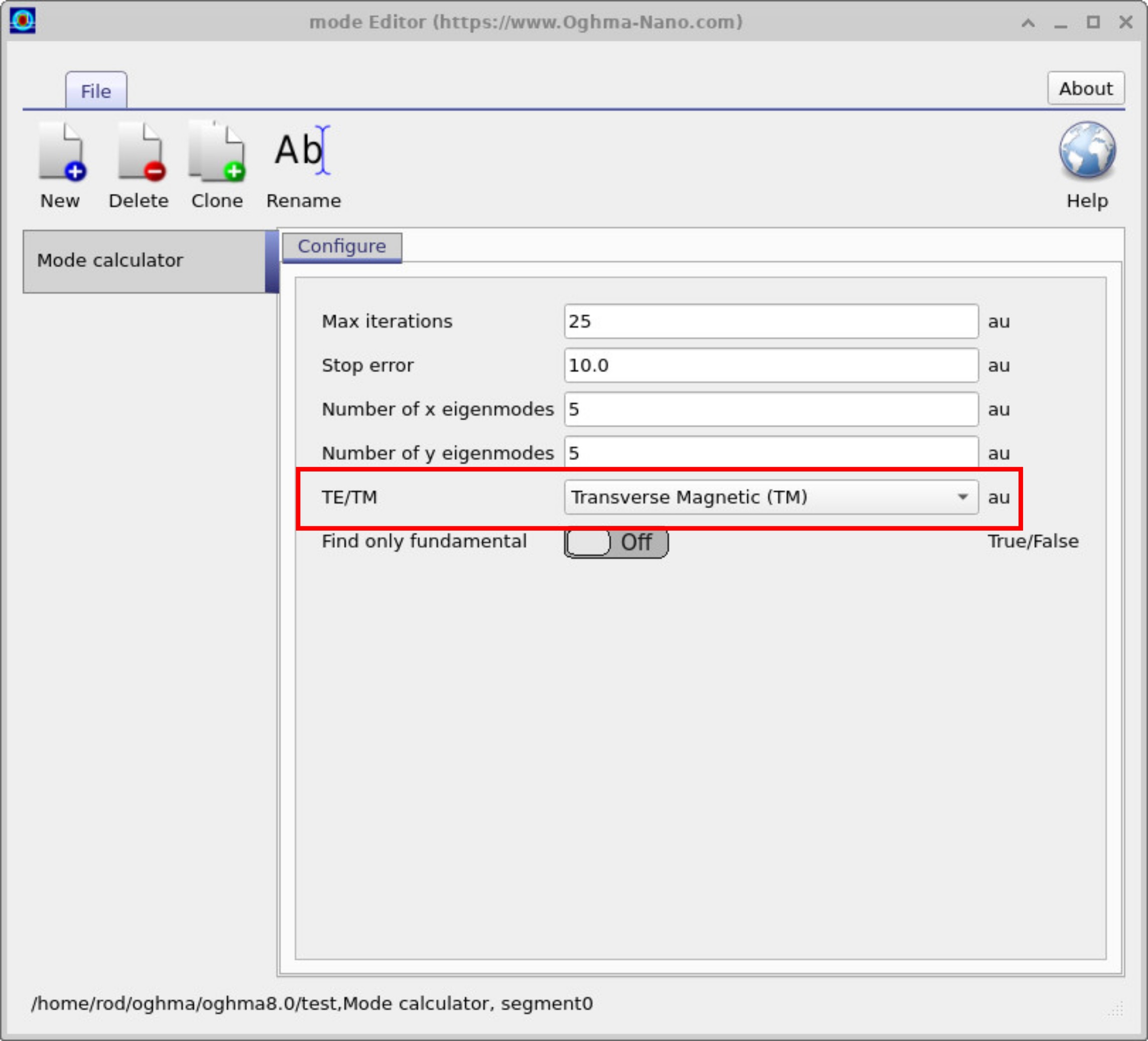
Clicking the Mode Calculator button opens the solver configuration window (??). Here you can set the maximum number of iterations, numerical tolerance, and the number of eigenmodes to search in the X and Y directions. The TE/TM selector allows you to switch between Transverse Electric and Transverse Magnetic calculations, which is useful for comparing how polarization affects the guided modes.