Part B: OLED simulation using ray tracing
1. Introduction
In the previous section we used the transfer matrix method (TMM) to compute the probability that photons escape the device. TMM treats light as a wave, naturally capturing multiple reflections at layer interfaces and the resulting interference within the thin-film cavity.
In this section we switch to a complementary approach: ray tracing. Here light is treated as particles (rays), which is the paradigm widely used in computer graphics. A key advantage is its explicit angular dependence: we can track how rays refract and reflect as they leave the device and therefore predict angle-resolved behavior—such as the colour (spectrum) observed as a function of viewing angle—which is the focus of this section.
2. Quick start - ray tracing
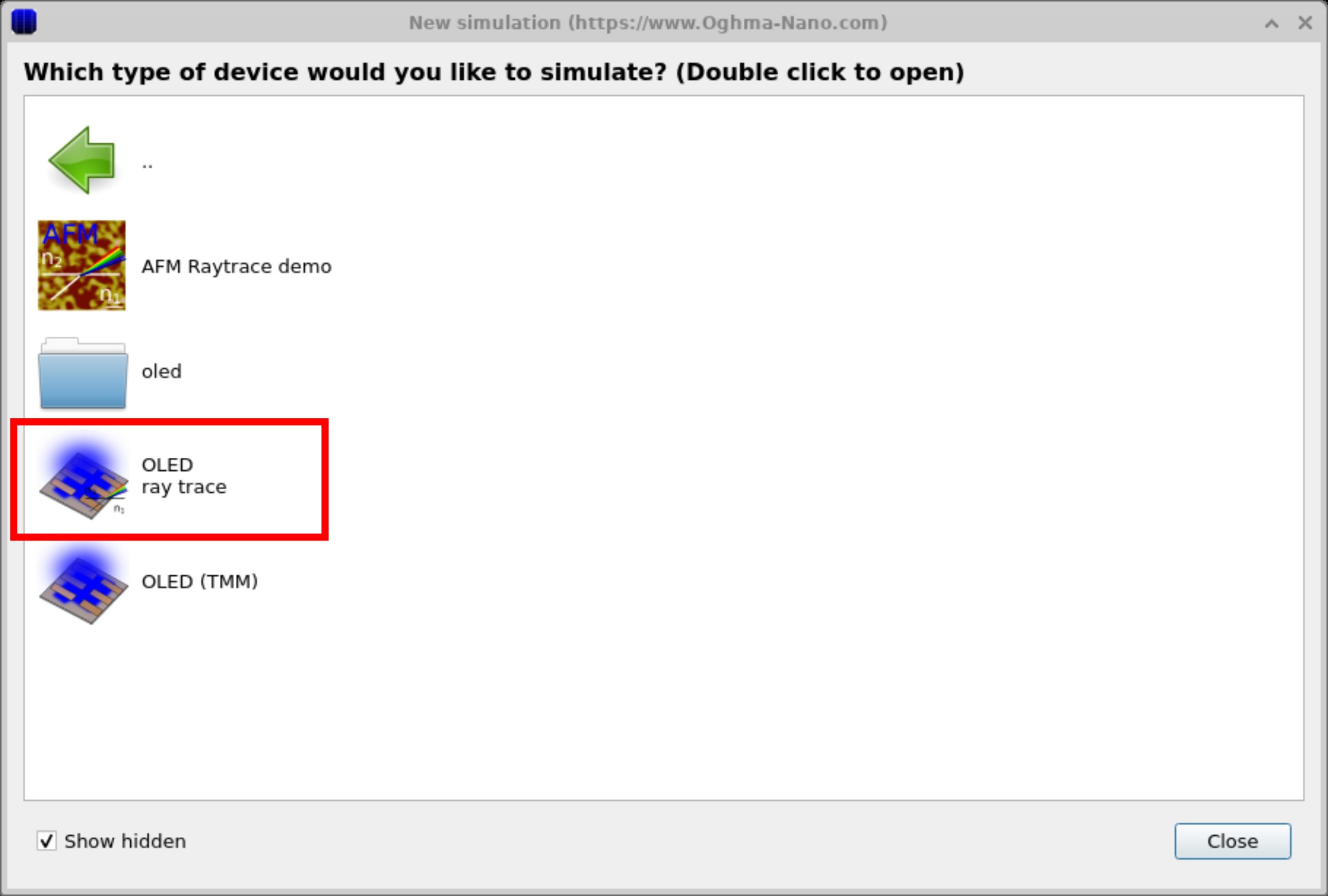
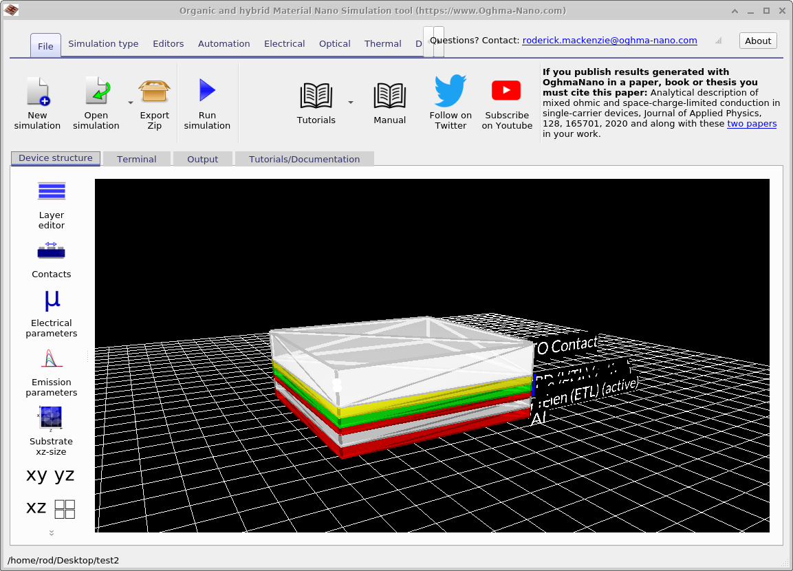
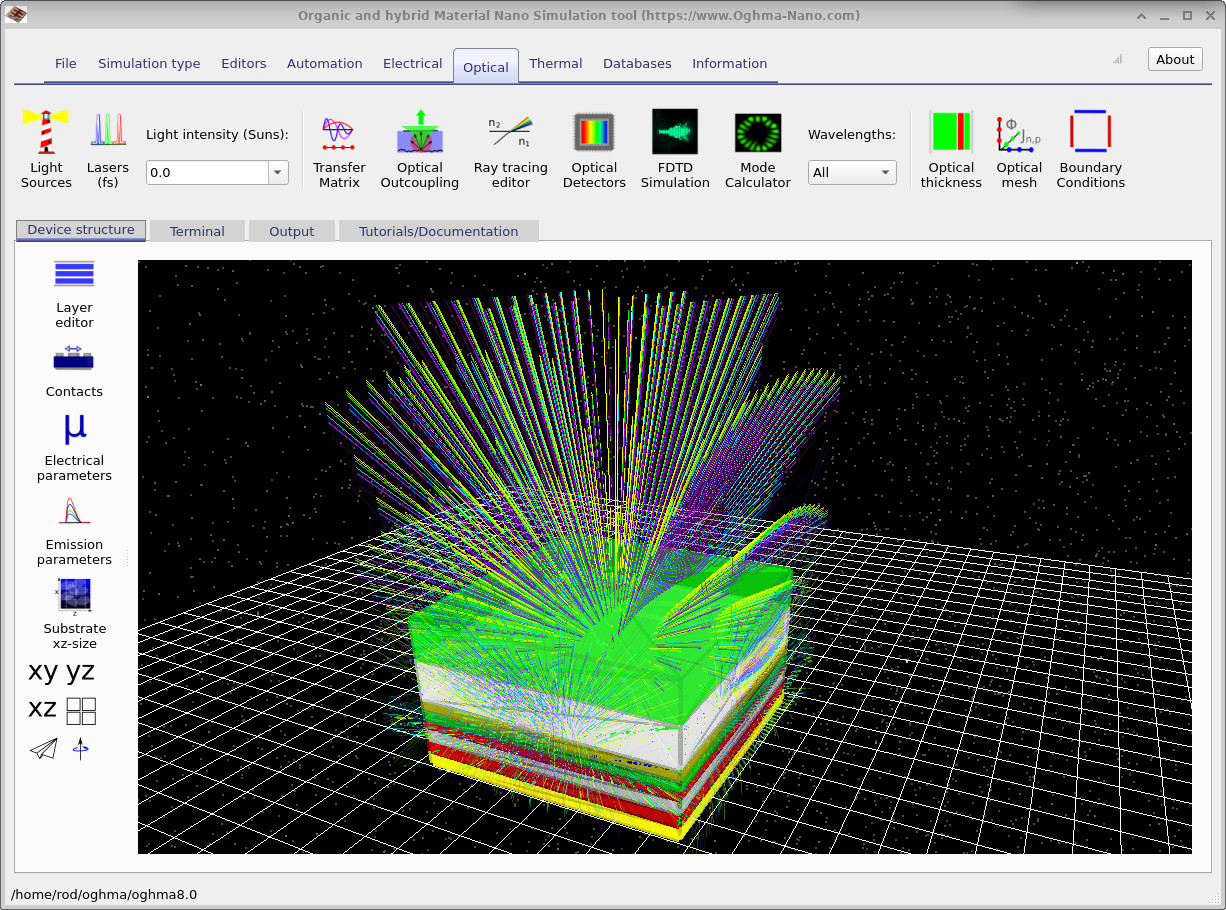
To create a new OLED ray-tracing simulation, open the New simulation window and double-click OLED (Ray Trace) (see ??). Save the new project to disk. After it opens, you’ll see the main OLED interface ( ?? ), which is similar to the previous example, but with the ray tracer enabled as the optical model.
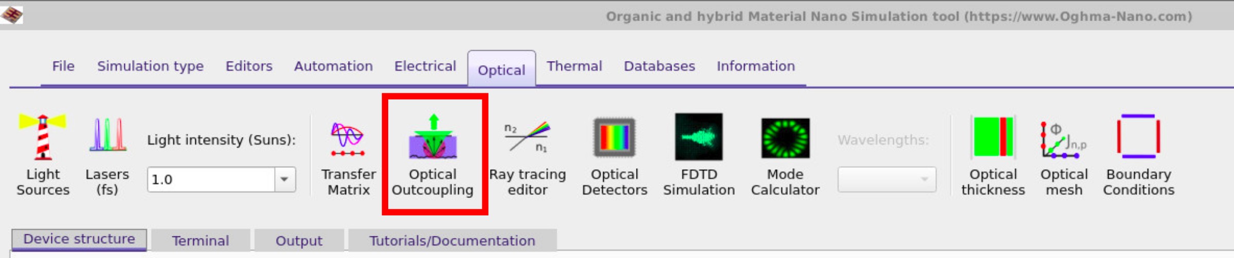
In the main interface, navigate to the Optical ribbon (??) and click on Optical outcoupling, just as in the previous simulation. This opens the outcoupling window (see ??). Notice that this time the Ray Trace button is selected in the main interface instead of the Transfer Matrix button. Clicking the Run optical simulation (▶) button will launch the ray tracer, which propagates rays from every mesh point within the active layer to calculate the probability that photons escape the device at each position.
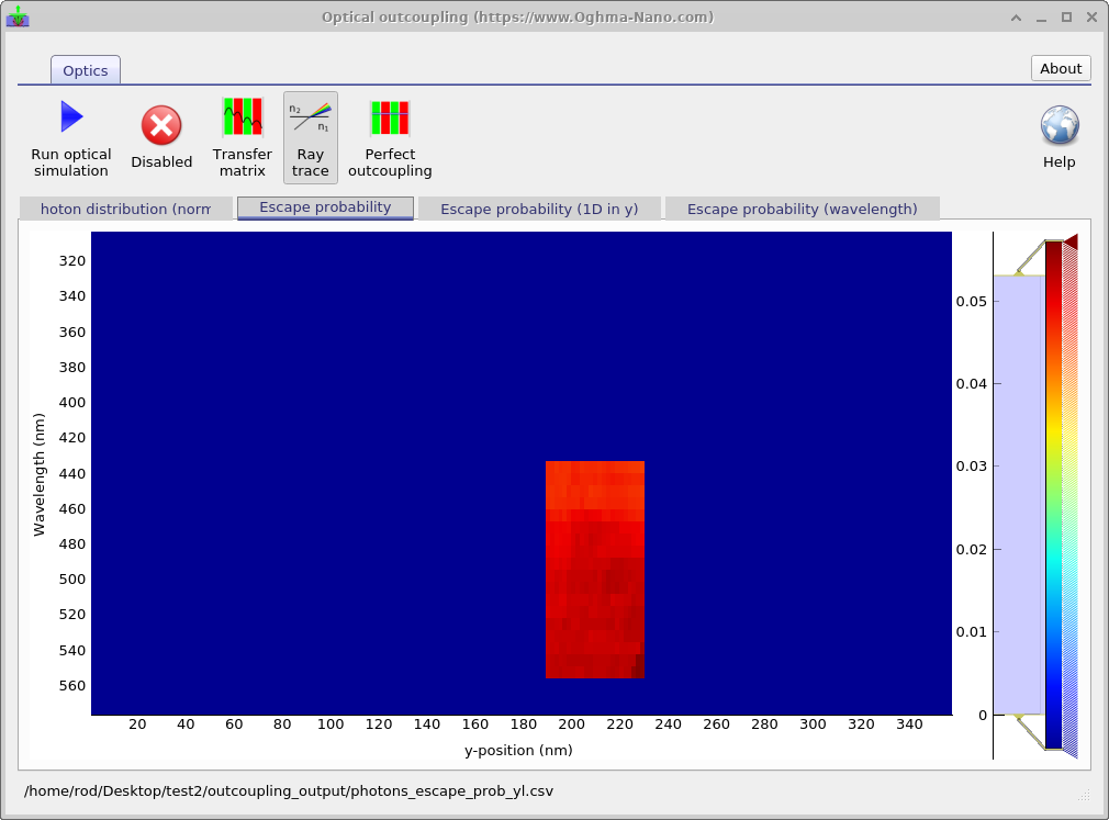
This will take much longer than TMM simulations due to the increased complexity. Also the simulations will only calculate the escape probability for the active area to save time. Note that the outcoupling efficiency for ray tracing is lower than that predicted by the transfer matrix as the transfer matrix method assumes propagation normal to the interfaces while ray tracing allows rays to travel in all directions some of which will never leave the device.
3. Electrical simulations combined with ray tracing
Now return to the main simulation window and press the blue Play button
(or press 9) to run the main simulation. This run first executes the
ray tracer and then the drift–diffusion solver. The ray tracer calculates
the probability that photons generated in the active layer escape the device, and it also
determines the emission angle distribution (hence which colours are visible at which angles).
The drift–diffusion solver then computes the magnitude of the emitted light by evaluating the
recombination term, which represents the radiative emission rate.
The resulting ray-tracing view is shown in
Figure 5,
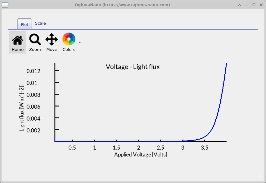
and the corresponding voltage–light output plot
(lv.csv, light vs. voltage) is shown in
Figure 6.
3. Key outputs
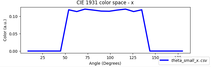
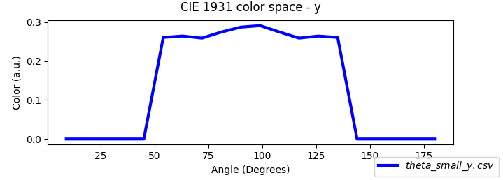
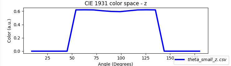
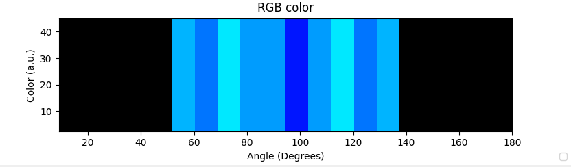
If you inspect the outputs of the combined ray-tracing and drift–diffusion simulation (??), you’ll see that many files match those described in the previous (transfer-matrix) section. The crucial addition is that ray tracing yields an angle-resolved emission profile, so OghmaNano also writes angle-dependent color data: the overall RGB versus viewing angle (theta_RGB.csv) and the CIE 1931 components x, y, z and tristimulus X, Y, Z versus angle (theta_x/y/z.csv, theta_X/Y/Z.csv). These appear as rainbow spectrum preview icons in the figure and are summarized in the table below.
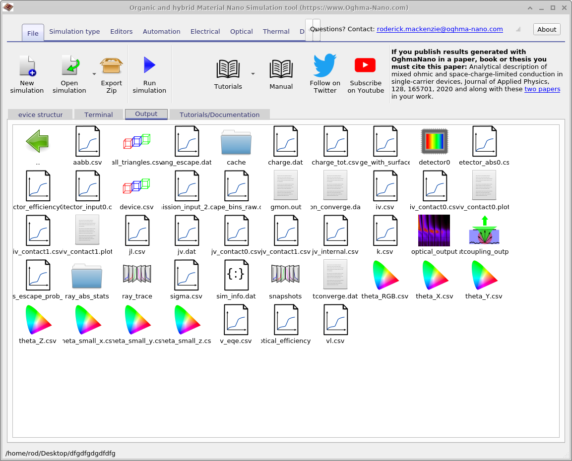
theta_RGB.csv, theta_x/y/z.csv, theta_X/Y/Z.csv, etc.).
| File name | Description |
|---|---|
theta_RGB.csv |
RGB values vs. viewing angle |
theta_x.csv |
CIE 1931 x vs. viewing angle |
theta_y.csv |
CIE 1931 y vs. viewing angle |
theta_z.csv |
CIE 1931 z vs. viewing angle |
theta_X.csv |
CIE 1931 X vs. viewing angle |
theta_Y.csv |
CIE 1931 Y vs. viewing angle |
theta_Z.csv |
CIE 1931 Z vs. viewing angle |
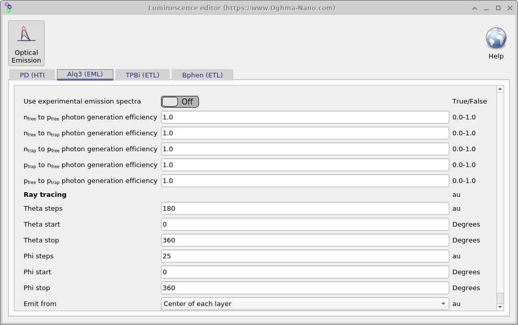
4. The spectrum of the emitted light
Just as you set electrical parameters per layer, you can configure the emission spectrum for each layer in the Emission parameters window (open it from Device structure → Emission parameters in the main interface; see Figure 5). The spectrum can be either:
-
Experimental spectrum — toggle Use experimental emission spectra On, then
choose a dataset via Experimental emission spectra. Control overall strength with
Experimental emission efficiency (range
0.0–1.0, au). Many datasets are available in the materials database, and you can add your own (see Databases). -
Calculated spectrum — toggle Use experimental emission spectra Off to
compute the spectrum from carrier populations and the density of states using Fermi’s Golden Rule. Additional
photon-generation efficiency terms appear (all
0.0–1.0, au): nfree→pfree, nfree→ntrap, ntrap→pfree, ptrap→nfree, and pfree→ptrap. This mode is intended for advanced users.
When Ray tracing is used for outcoupling, each layer can specify emission directions under the
Ray tracing section using spherical angles:
Theta steps (e.g. 180), Theta start/stop (degrees, e.g. 0–360);
Phi steps (e.g. 25), Phi start/stop (degrees, e.g. 0–360). This lets you
explore angular light escape. For flat, laterally uniform stacks, symmetry often means you only need to vary one of
theta or phi.
The Emit from option controls ray source positions: Center of each layer launches rays from the middle of each emission layer (fast); At each electrical mesh point launches rays at every electrical node for higher fidelity (slower, but can be offset by increasing the number of threads).
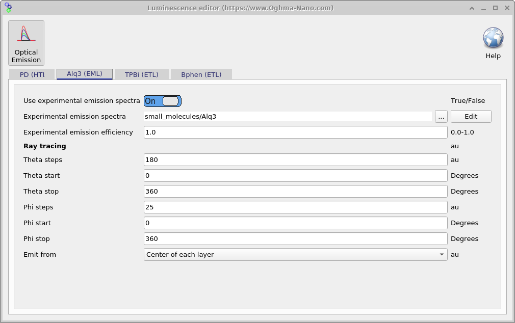
small_molecules/Alq3), set efficiency, and configure angular sampling for ray tracing.