Advanced fitting techniques
1. Choosing the right minimizer
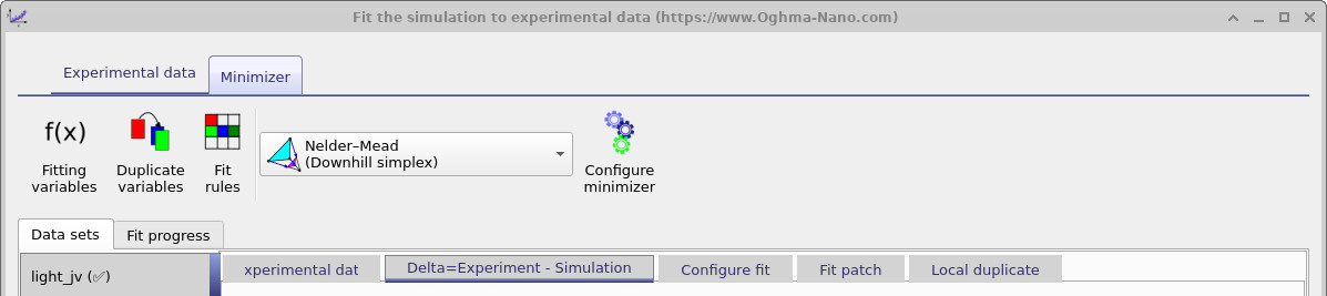
The Minimizer ribbon is where you choose and configure the algorithm that drives the fitting process. Selecting the right minimizer can make the difference between a fast, robust convergence and a slow or unstable fit. OghmaNano provides several well-established algorithms, each with different strengths, which can be selected from the Fitting method drop-down menu.
Broadly speaking, fitting algorithms fall into two categories. The first are downhill or gradient-based methods, which try to “roll a ball down a hill” until it reaches the minimum error. Some of these require explicit gradient calculations, which can be costly and fragile for complex models; others are derivative-free and usually more robust. The second category are statistical methods, which do not only seek the best fit but also provide a probability distribution that indicates the confidence and uniqueness of the solution. These methods are more computationally demanding but can give deeper insights into parameter uncertainty.
| Method | Downhill | Gradient | Statistical | Comment |
|---|---|---|---|---|
| Nelder-Mead | ✅ | ❌ | ❌ | Robust, slow, reliable |
| Newton | ✅ | ✅ | ❌ | Fragile, sometimes fast |
| Thermal Annealing | ❌ | ❌ | ✅ | Surprisingly good |
| MCMC | ❌ | ❌ | ✅ | ? |
| HMC | ❌ | ❌ | ✅ | ? |
Nelder–Mead (Simplex Downhill)
The Nelder–Mead simplex algorithm is the most widely used fitting method in OghmaNano — in fact, all published papers up to 2024 relied on it. A general introduction to the method can be found here: https://en.wikipedia.org/wiki/Nelder%E2%80%93Mead_method . In practice, this minimizer is robust and does not require gradients, making it well suited to complex problems. Its main configuration options are:
- Stall steps: Stops the fit if the error does not improve after the specified number of steps.
- Disable reset at level: Prevents the algorithm from restarting once the error has fallen below the defined threshold.
- Fit convergence: Defines the error level at which the fit is considered converged and the run terminates.
- Start simplex step multiplier: Sets the size of the initial parameter perturbation. Values > 1.0 encourage wide exploration of parameter space; values < 1.0 keep the fit close to the initial guess. As a rule of thumb, 2.0 is “large” and 0.1 is “small.”
- Enable snapshots during fit: By default snapshots are disabled to reduce disk access. Turning this on forces snapshots to be saved at each step, but slows performance.
- Simplex reset steps: Specifies how many steps are taken before the simplex is reset. Resetting can help escape local minima but may also push the solution away from convergence.
The main advantage of Nelder–Mead is its simplicity and robustness. Conceptually, it “rolls a ball downhill” toward the minimum error surface without requiring gradient calculations, which is particularly valuable for noisy or discontinuous models.
💡 Practical tips for using Nelder–Mead
- We recommend starting with Nelder–Mead for most fitting problems. Only switch to other minimizers if convergence fails or you need statistical insights.
- This method was used in all OghmaNano papers published up to 2024, making it a proven and reliable baseline for reproducibility.
- Nelder–Mead can be slow for high-dimensional problems (i.e. when fitting many variables at once).
- Always minimize the number of fitting variables to those strictly needed — this reduces dimensionality and improves convergence.
- Run One iteration first to check sensitivity before committing to a full automated fit.
Thermal Annealing
Thermal annealing is a stochastic optimization method inspired by the physical process of cooling a material from high temperature to low temperature. In OghmaNano, this algorithm explores the parameter space defined by the variable limits you specify. Correctly setting those bounds is essential — the minimizer will not search beyond them.
In practice, thermal annealing often performs surprisingly well and can be faster than Nelder–Mead at finding a reasonable solution. However, the final fits are sometimes less precise or “polished,” and additional refinement with Nelder–Mead may still be needed. Thermal annealing is particularly useful for escaping local minima and performing global exploration of the parameter space.
- Dump every n steps: Saves the current state to disk at the specified interval.
- Cooling constant: Controls how quickly the simulated “temperature” decreases. The cooling follows \( e^{-k(T_{\text{start}}-T_{\text{stop}})} \), where \(T_{\text{start}} = 300\,K\) and \(T_{\text{stop}} = 0\,K\).
- Annealing steps: Number of iterations used to cool the system from \(T_{\text{start}}\) to \(T_{\text{stop}}\).
💡 Tips for using Thermal Annealing
- Best used when Nelder–Mead gets stuck in a local minimum.
- Set parameter bounds carefully — the algorithm will not search outside them.
- Expect quicker convergence than Nelder–Mead, but with less accurate final results.
- Consider running Nelder–Mead afterwards to refine the solution obtained by annealing.
Newton
Newton’s method is included in OghmaNano for completeness, but it is rarely the best choice for most fitting problems. As a gradient-based minimizer, it requires derivatives to be calculated at each step. While this can occasionally make it faster than Nelder–Mead for certain smooth, well-behaved problems, it also makes the algorithm fragile: small numerical errors in derivative evaluation can cause the fit to diverge or stall.
In practice, Newton’s method is highly sensitive to the initial guess and the scaling of variables. Unless the problem is very simple and well-conditioned, convergence is often poor. For these reasons, it is generally not recommended as a primary method but can be useful as a diagnostic tool or for experimentation in controlled cases.
💡 Tips for using Newton’s method
- Only use Newton on small, smooth problems where good initial guesses are available.
- Ensure that variable ranges are well scaled — poor scaling can cause divergence.
- If Newton fails to converge, fall back to Nelder–Mead or thermal annealing.
- Consider Newton mainly for testing or exploring specific cases, not for production fitting.
Markov chain Monte Carlo (MCMC)
Markov chain Monte Carlo (MCMC) is a statistical fitting method that samples parameter space randomly but in a way that builds up the correct probability distribution over time. Unlike Nelder–Mead or Newton, which return a single “best-fit” set of parameters, MCMC produces a distribution of solutions that shows how probable different parameter values are. This makes it particularly powerful for quantifying uncertainty and identifying correlations between variables. In OghmaNano, support is implemented but has not been robustly tested.
Hamiltonian Monte Carlo (HMC)
Hamiltonian Monte Carlo (HMC) extends the MCMC idea by using gradient information to propose more efficient jumps through parameter space. Instead of moving randomly, HMC simulates the “motion” of a particle through the likelihood landscape, guided by gradients, which can dramatically improve sampling efficiency in high-dimensional problems. Like MCMC, HMC generates a probability distribution over fitted parameters rather than a single solution. In OghmaNano, support is implemented but has not been robustly tested.
No-U-Turn Sampler (NUTS)
The No-U-Turn Sampler (NUTS) is an adaptive variant of HMC that automatically decides when to stop a trajectory through parameter space to avoid wasted computation or retracing paths. This makes NUTS more user-friendly, since it reduces the need to manually tune algorithm parameters. NUTS is widely regarded as one of the most efficient and robust methods for Bayesian parameter estimation. In OghmaNano, support is implemented but has not been robustly tested.
👉 Next step: Now continue to Part C for more advanced fitting methods.