🎯 Learning objectives

Load experimental JV data into OghmaNano and prepare it for fitting.
Configure fitting variables, bounds, and constraints to guide the minimizer.
Run single-iteration and automated fits, and interpret error functions and convergence plots.
Apply duplicate variables and fit rules to enforce symmetry and physical consistency.
Extract meaningful device parameters (e.g. mobilities, resistances, trap densities) from fitted data.

📦 Prerequisites

OghmaNano installed and working.
Basic familiarity with solar-cell concepts.

⏱ Estimated time

Part A: 10-15 min
Part B: 10-15 min
Part C: 10-15 min

🎥 Related YouTube Videos

Advanced fitting techniques

How the fitting process works

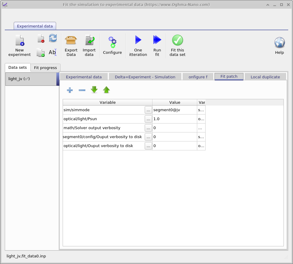
When you click the "Run fit" button, OghmaNano makes a new directory inside the simulation directory called "sim" this is the directory in which the fitting process takes place. Inside this directory OghmaNano will make one new directory for each data set you are trying to fit, it will populate each directory with the sim.json (and sim.oghma) files from your main simulation directory. At this point the sim.json files in all the directories are identical. Then using the contents of the fit "fit patch" (see figure 16.12) the content of each sim.json file will be updated, this process is called patching the simulation files. This process enables you to adjust parameters in each simulation directory to match the data set you are trying to fit. For example you might want one data set to have optical/light/Psun set 1.0 and another to be set to 0.0 to enable fitting of a 1 sun JV curve and a dark JV curve. After patching each directory, the fitting process then commences. During this process fitting variables in the sim.json files in the "sim" directory are updated. During the fit the algorithm will often produce fits which are worse than the current best effort, and only sometimes produce fits which are better than the current best effort. Only when a better fit is obtained will the sim.json file be updated in the main simulation directory and the curves in the GUI also updated.

Fitting without the GUI

The GUI is a very easy and efficient way to setup a fit. However, it takes considerable CPU time to update the user interface as the fit runs and this therefore slows the fitting process. Therefore if you are doing lots of fitting or fitting difficult problems, fitting without the GUI can be faster. This section covers how to fit from the Windows command line:

First set up your simulation you want to fit in the usual way using the GUI. Run a single iteration of the fit to make sure it looks right. Then close the GUI.
Next we need to tell Windows where it can find OghmaNano, usually it has been installed in C:\Program files x86 \OghmaNano . If you open this directory you will see lots of files. But the two key ones are oghma.exe and oghma_core.exe. The file oghma.exe is the GUI, oghma_core.exe is the core solver, these are completely independent programs. The core solver can be run without the GUI. To tell windows where these files are we need to add C:\Program files x86 \OghmaNano to the windows path. This can be done by following these https://docs.microsoft.com/en-us/previous-versions/office/developer/sharepoint-2010/ee537574(v=office.14) instructions. These instructions are for a modern version of Windows, but on your system things may be in slightly different places. On most versions of windows the process is more or less the same, if you get stuck google "adding a path to window".
Click on the start menu and type "cmd" and enter to bring up a Windows terminal. Type:
```
oghma_core.exe --help
```
Note it is a double dash before help not a single dash.

This should bring up some help for OghmaNano. If it does them we have successfully told windows where oghma_core.exe lives. If you get an error, try step 2 again (and/or restart your computer).
Now that windows knows where oghma_core.exe lives, we can navigate to our simulation directory. Use cd to navigate to the directory where your simulation you want to fit is saved.
First run the command oghma_core.exe to see if your simulation runs OK. If it does not then recheck your simulation file.
Now run a single fit by typing:
```
oghma_core.exe --1fit
```
Inspect the results in the "sim" directory, use your favourite plotting program to compare the results to the experimental data. Note the experimental data is stored in fit_data(0-1).inp.
If everything went well with the above step, you can run a real fit by typing:
```
oghma_core.exe --fit
```
Again those are double dashes before the fit command. Ctrl+C will terminate the fit. You can check the progress of convergence by plotting fitlog.csv.