Fitting experimental data
1. Overview
Just as you can fit the diode equation to a dark JV curve to extract the ideality factor, OghmaNano lets you fit full device models directly to experimental data. By calibrating the simulation to your measurements, you can recover physically meaningful parameters—mobilities, trap-state densities, contact resistances, recombination coefficients—within a self-consistent framework. Compared with simple analytical formulas, a physics-based fit preserves optical–electrical coupling and provides richer, more reliable insight into the mechanisms that govern performance. This tutorial introduces the fitting workflow in OghmaNano and shows how to choose variables, select minimizers, and run efficient, reproducible fits.
2. Your first fit
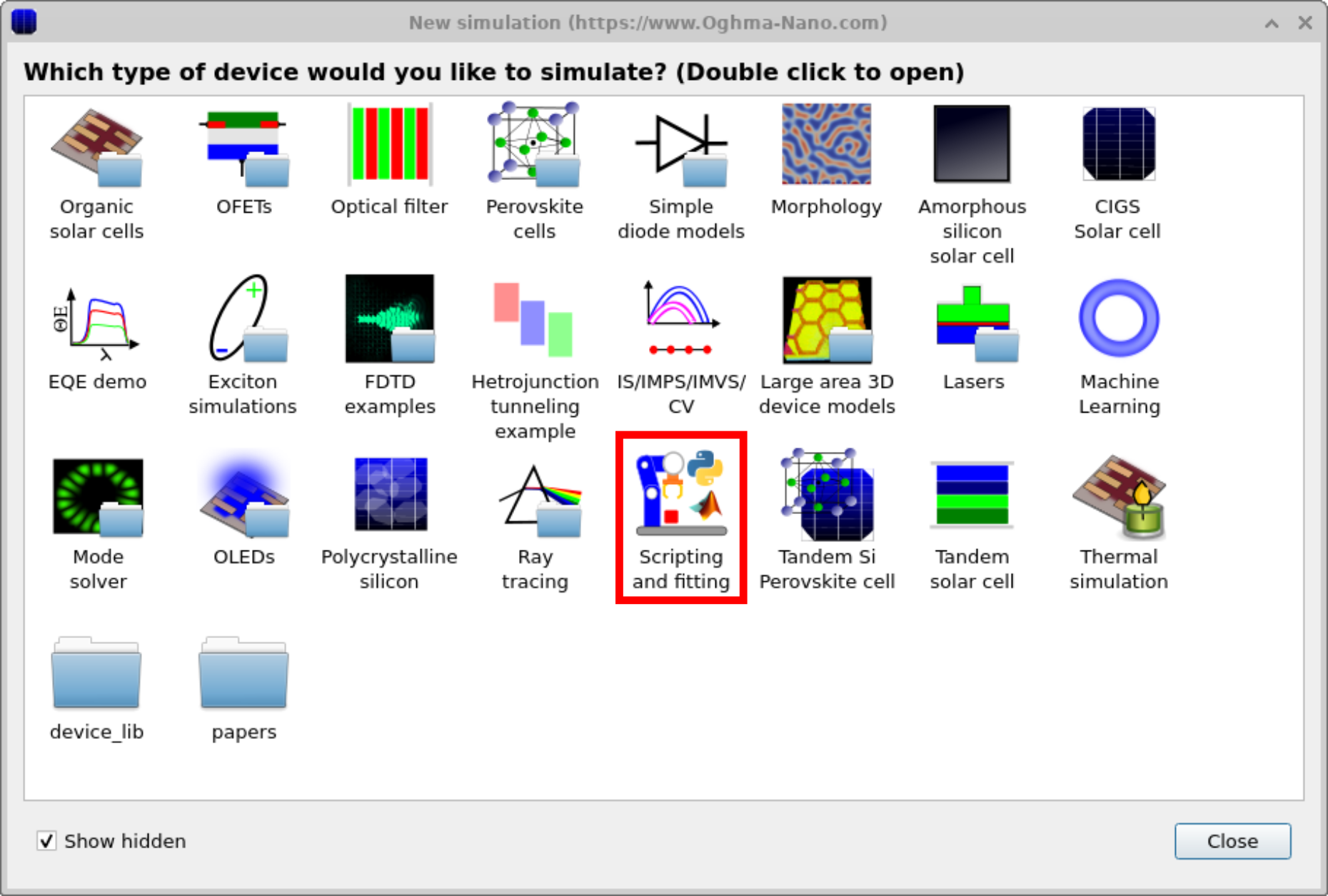
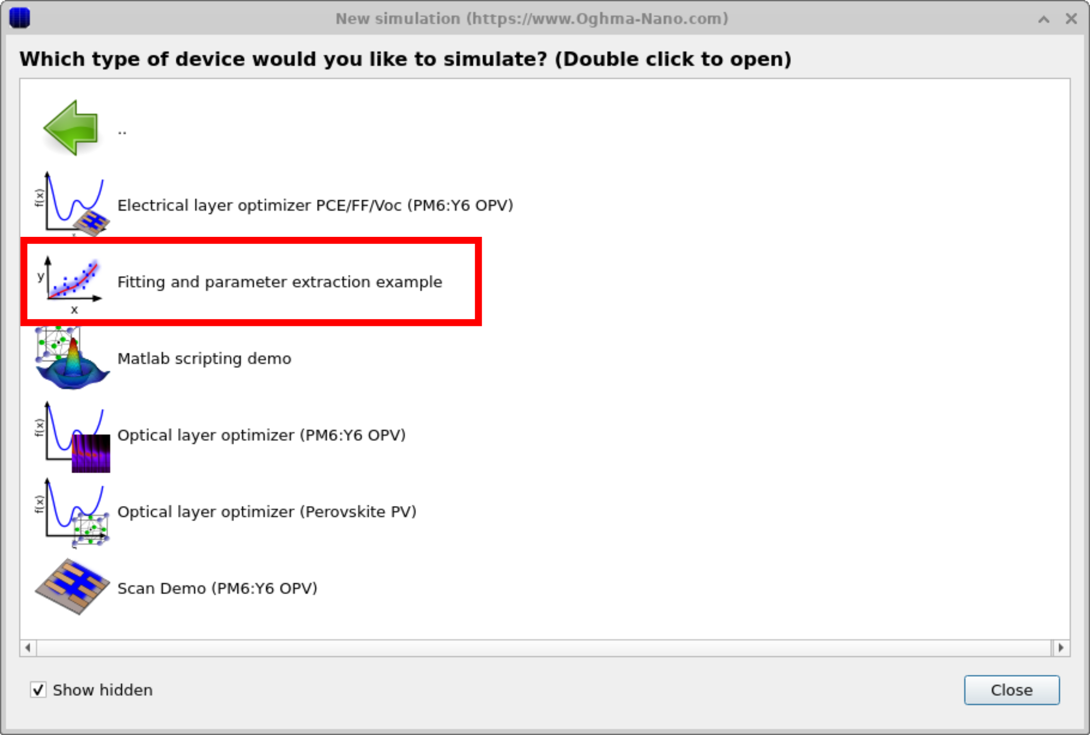
OghmaNano includes several demo simulations that illustrate how to fit models to experimental data. One of these uses a simple drift–diffusion model as an example. To access it, click the New simulation icon in the File ribbon to open the New simulation window (Figure ??). From here, double-click the Scripting and fitting category to open the folder shown in Figure ??. Select the Fitting and parameter extraction example to load a demonstration project. When opened, it launches a simple solar-cell simulation (Figure ??). Although this demo focuses on a solar cell, the fitting engine can be applied to any simulation and experimental data set.
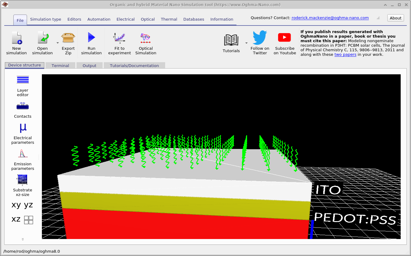
Once you have saved the new simulation, the main simulation window will appear (??). From here, navigate to the Automation ribbon (highlighted in red) and select the Fit to experiment icon to access the fitting window ??.
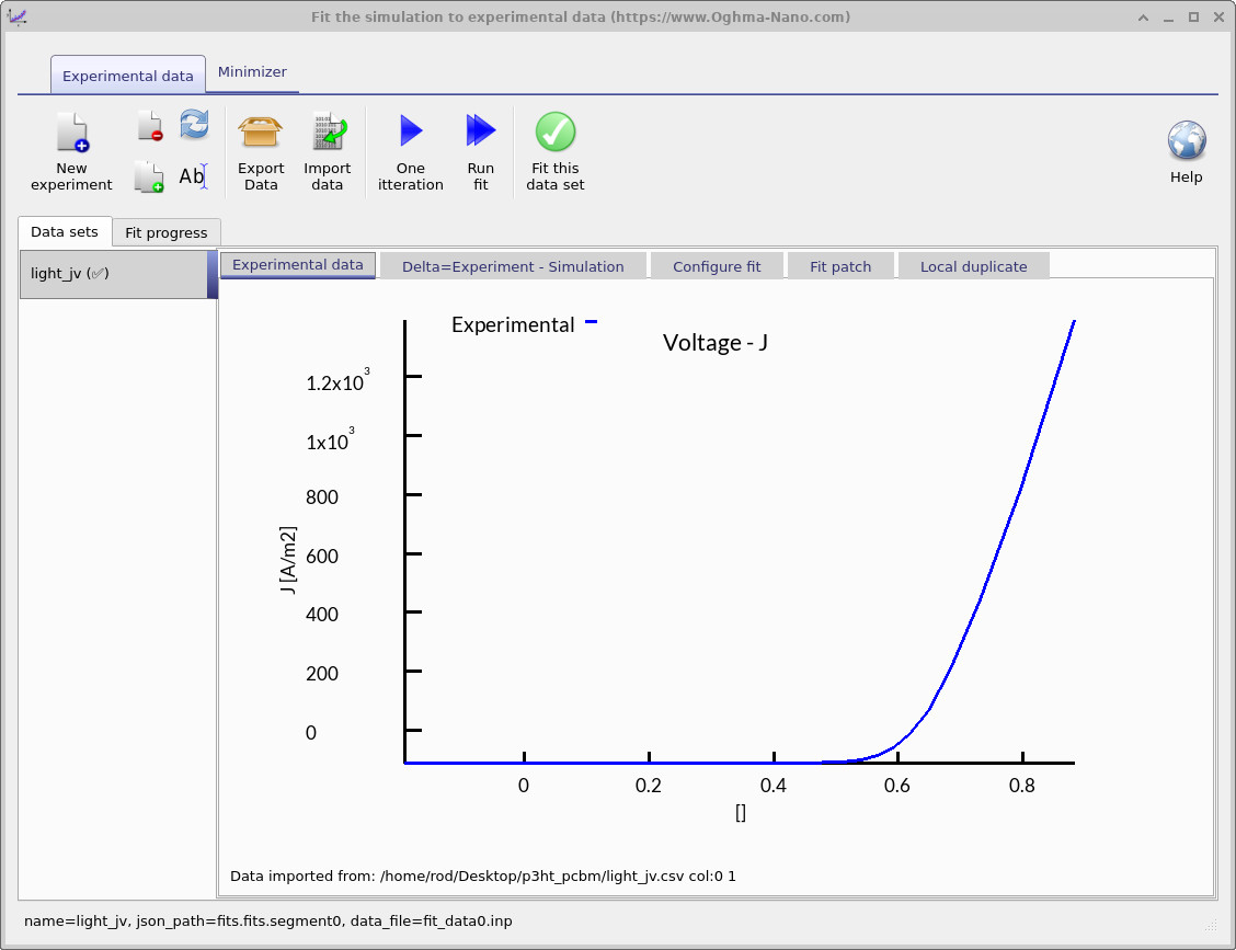
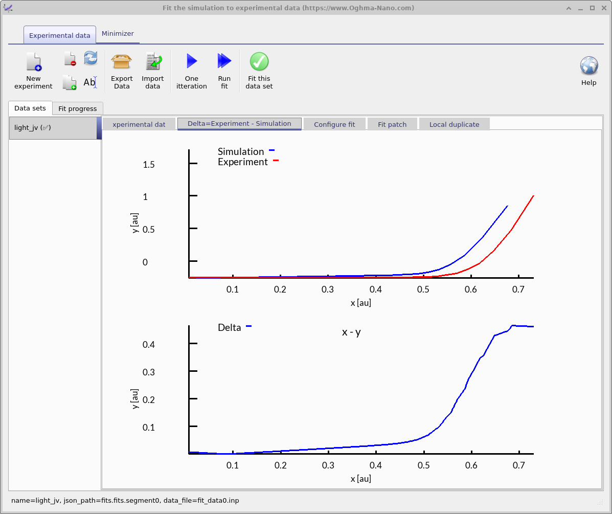
The fitting window controls how the optimization is performed: it specifies which experimental data sets are used and which simulation variables are adjusted. You can fit to a single data set, as shown here, or to multiple data sets simultaneously for more constrained parameter extraction. In Figure ??, the blue line represents the experimental JV curve that will be used for fitting.
💡 Practical exercise: Using the fitting window
- Task 1 – One iteration: Click the One iteration button to update the fitting view (??a). In the Delta = Experiment − Simulation tab you’ll see the simulated JV (blue) overlaid on the experimental JV (red), plus the green delta curve defined point-by-point as \( \Delta(V) = J_{\mathrm{exp}}(V) - J_{\mathrm{sim}}(V) \). A good starting point is when the green curve is close to zero across the voltage range.
-
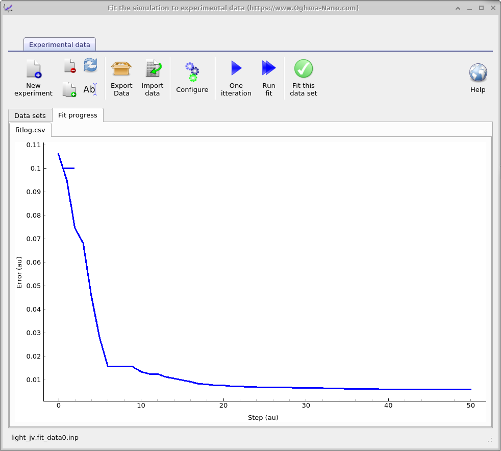
Task 2 – Run fit:
Press Run fit to launch the automated minimizer (pressing it again stops the run).
During the first few steps the error may briefly increase, but it should then fall as the simulated and
experimental curves converge. Switch to the Fit progress tab to plot the error versus iteration
(??b); this graph is also
saved to
fitlog.csvin the simulation directory for external plotting. On a typical setup this stage takes ~30 s.
3. Adding and removing data
The main fitting window provides a toolbar of commands that control how experiments are added, managed, and fitted. These buttons let you import or remove data sets, configure which parameters are varied, and start or stop the fitting process. The most important options are:
- New experiment: Adds another experimental data set to the fitting window. For example, you can include both a light JV curve and a dark JV curve. Fitting against multiple data sets improves the reliability of extracted parameters, but also makes the fitting process slower and more challenging.
- Delete experiment: Removes the selected data set from the fit.
- Clone experiment: Creates a duplicate of the current data set.
- Rename experiment: Allows you to rename the selected data set.
- Export data: Saves the current fit and data as a compressed zip file.
- Import data: Loads external experimental data into the fitting window (see the Import Wizard section for details).
- Configure: Opens the configuration window for defining which variables will be adjusted during fitting (explained in detail below).
- One iteration: Runs a single fitting step to check how close the simulation is to the experimental data. It is recommended to use this option and adjust parameters manually until you have a reasonable starting point before running the automated fit.
- Run fit: Starts the automated fitting algorithm. The process continues until stopped manually by pressing the button again.
- Fit this data set: Enables or disables fitting for the currently selected data set.
4. The minimizer ribbon
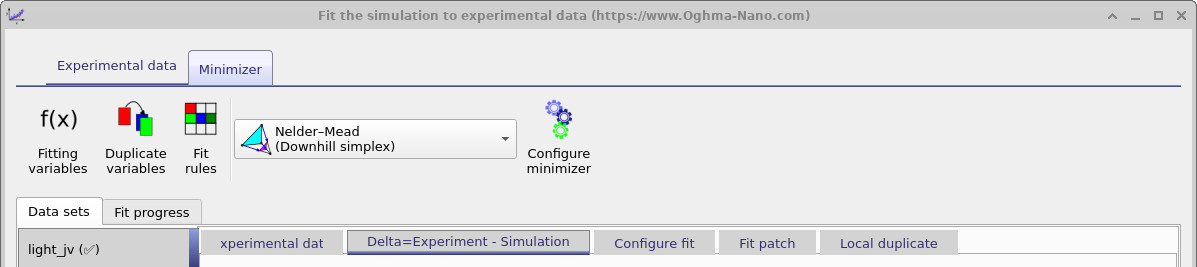
The Minimizer ribbon provides control over the optimization algorithm used during fitting. From this tab you can choose which minimizer to apply (for example, the default Nelder–Mead downhill simplex) and configure its settings. The ribbon also includes tools for managing fitting variables, duplicating parameters, and applying mathematical rules to constrain the fit. By adjusting these options, you can control how the algorithm explores parameter space, balance speed against accuracy, and ensure that physically meaningful constraints are enforced during the fitting process.
5. Setting the variables to fit
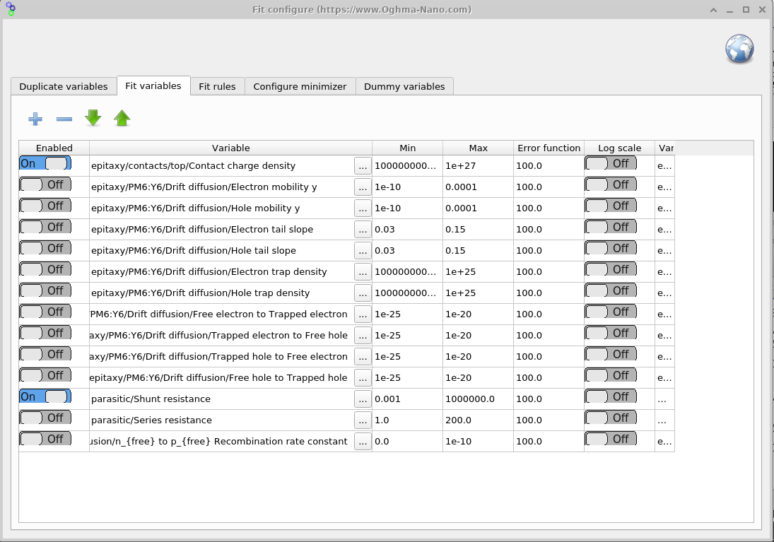
To open the Fit variables window, go to the Minimizer ribbon in the fitting window (Figure ??) and click Fitting variables. This panel (Figure ??) lets you choose which parameters are varied during the fit and set their bounds. For speed and robustness, start with a small set of symmetric parameters; add more (or introduce asymmetry) only after you have a reasonable initial fit.
The Fit variables table contains seven columns: Enabled, Variable, Min, Max, Error function, Log scale, and Variable (JSON).
- Enabled: Turns the fitting of the variable on or off.
- Variable: Describes the path of the variable to be fitted in English.
- Min: The minimum value the variable can take.
- Max: The maximum value the variable can take.
- Error function: Penalty added to the total fitting error if the variable strays outside its min–max range. This effectively pushes the algorithm back into the allowed bounds.
- Log scale: Fits the parameter on a logarithmic scale. Useful for variables that span many orders of magnitude to ensure the whole range is explored.
- Variable (JSON): Usually hidden; represents the full path of the parameter in
jsonformat. The backend uses this path, while the English path is only for readability and may not always be exact.
6. Duplicating variables
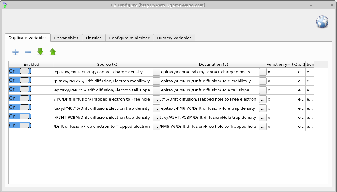
Open the Duplicate variables window from the Minimizer ribbon (??). This tool mirrors a source parameter to a destination parameter on every iteration. In the symmetric-device example, we fit only the electron-side parameter and use Duplicate variables to copy its value to the corresponding hole parameter, keeping them equal throughout the fit (see ??).
The column Function y = f(x) defines how the source value x is transformed before it is
written to the destination y. The default x performs a direct copy; examples such as
2*x (double the value) or x + 0.05 (apply an offset) are also possible.
7. Fit rules
The Fit rules window (??), accessed from the Minimizer ribbon, allows you to apply mathematical constraints to the fitting process. Rules add a penalty to the error function whenever a condition is violated. For example, you can enforce that one parameter must always be larger than another, or apply a penalty if a variable drifts outside an acceptable range. This helps keep the fit physically meaningful and prevents the minimizer from exploring unrealistic parameter combinations.
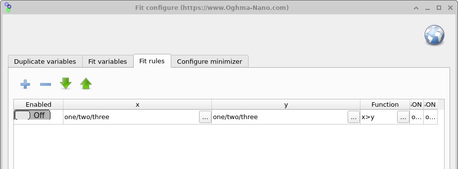
x > y to enforce
relationships between parameters. If a rule is broken, an additional error is added to the fit, guiding the
minimizer back into a valid region of parameter space.
💡 Key Tips and Tricks for Fitting:
- Generally speaking, fitting is a tricky process requiring a lot of patience and manual fine-tuning. Don’t expect to click a button and for it to just work — you will need to work carefully to get nice fits.
- If the fit is not working, something may be wrong with the physical assumptions you have made about your device. The model will only fit physically reasonable data, so if something is off by an order of magnitude, reconsider what you are asking the model to do. For example, if you just can’t get \(J_{sc}\) to match in a solar cell, could it be that your material is simply not absorbing enough photons to achieve your desired \(J_{sc}\) value?
- Different data sets provide different types of information. For example, the dark JV curve of a solar cell gives insights into shunt resistance, series resistance, and some mobility/recombination details. The light JV curve, however, provides almost no information about shunt resistance, so don’t expect it to give accurate estimates of \(R_{shunt}\). Always think about what information your data contains before interpreting fitted parameters.
- The fitting process works by: 1) running a simulation; 2) calculating the difference between numerical and experimental results; 3) tweaking parameters; 4) rerunning the simulation and checking if the error reduces; 5) if the error reduces, the parameter change is accepted and the process repeats. This can take hundreds or thousands of iterations. Therefore, individual simulations must run quickly. For example, if your mesh has 1000 points, try reducing it to 10 for fitting; if you have 1000 time steps, reduce to 100. Every speedup in the base simulation speeds up the fitting process.
- Writing files to disk is the slowest part of any computational process. Even modern SSDs are about 30× slower than main memory (e.g. 456 MB/s vs 12,800 MB/s for PC3-12800). Using USB drives, network storage, or cloud services like OneDrive/Dropbox makes this even worse. For speed, always save simulations to a local SSD (not a network or mechanical drive).
- Minimize the number of files your simulation produces. Turn off unnecessary outputs such as snapshots, optical output, or dynamic folders. A well-configured simulation should only produce about 50 files. If you see hundreds, investigate why.
- Although fitting can be done in the GUI, it is often slow. A good practice is to set up the fits in the GUI but run them from the command line (instructions are given below).
- Since fitting writes many files to disk, antivirus software can slow things down by scanning each file. Consider excluding your simulation folder from real-time scanning if this becomes an issue.
👉 Next step: Now continue to Part B for more advanced fitting methods.