Generating Machine Learning Data Sets

This chapter describes how to generate machine-learning datasets using OghmaNano. Typically, these datasets are exported and processed using external frameworks such as TensorFlow for training, inference, or prediction.

1. Introduction

It is often desirable to extract physical device parameters from experimental data using modelling. For example, one may have a set of JV curves and wish to determine the charge-carrier mobility and recombination rate of the device. Traditionally, this is achieved by fitting a physics-based model, such as OghmaNano, to the data (as described in the fitting tutorial). The drawback of this approach is that fitting a single data set can be time-consuming, and the difficulty increases substantially when multiple data sets must be analysed. The fitting process is complex, typically requiring significant expertise in numerical simulation and a considerable amount of manual intervention. As a result, detailed device fitting is only performed by a relatively small subset of the community.

A more modern approach is to use machine learning. Rather than fitting a single JV curve directly, a simulation is first constructed that represents the device structure. Instead of optimising individual electrical parameters, many thousands of copies of this device are generated with randomly selected parameter values. Each of these instances is referred to as a virtual device. A simulation program such as OghmaNano is then used to generate JV curves for each virtual device, producing a data set consisting of JV curves paired with their corresponding electrical parameters. This data can be used to train a machine-learning model to predict electrical parameters directly from JV characteristics. In this framework, OghmaNano acts as a forward transform, mapping electrical parameters to simulated experimental data, while the machine-learning model provides the inverse transform. Once trained, the model can be applied to extract material parameters from real devices.

The key advantage of this approach is that, once trained, the machine-learning model can extract material parameters from experimental data within seconds, without requiring the user to be an expert in numerical simulation. However, the success of this method depends critically on the generation of a large, high-quality training data set. The process of constructing such data sets using OghmaNano is described in the following pages.

2. Opening the example

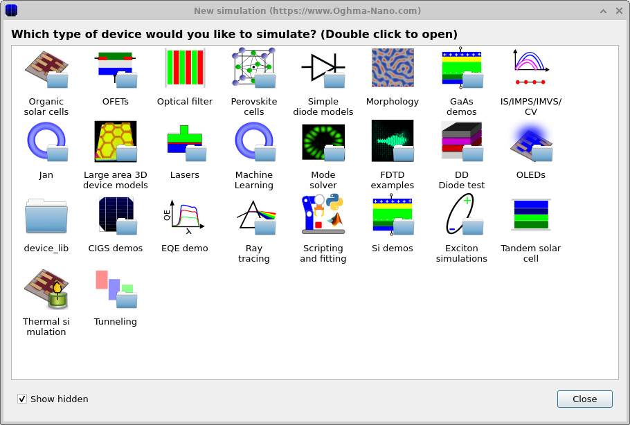
The example discussed on this page can be accessed via the New simulation button in the main window. This opens the New simulation browser shown in ??.

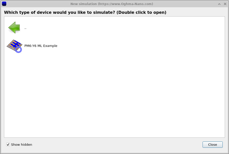
From the list of available simulation categories, double-click Machine learning to display the machine-learning examples (??). Selecting the PM6:Y6 ML example loads a preconfigured simulation corresponding to the device and workflow discussed in this chapter.

Once opened, the simulation presents the same device structure and automation setup used throughout this section, and can be used directly to generate machine-learning training data without further configuration.

3. Defining the simulations and output vectors

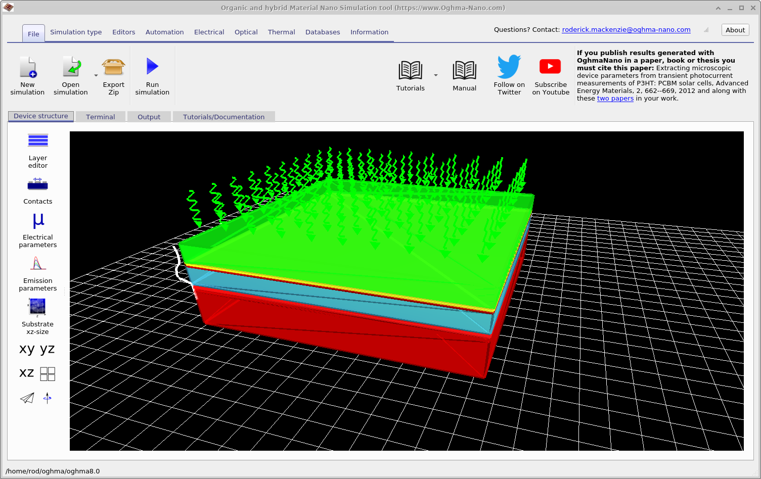
Once the example simulation has been opened, you will be presented with the main simulation window shown in Figure ??. This window shows the fully configured device structure used throughout this chapter. In the Automation ribbon, a Machine learning icon is visible, represented by a blue circular symbol. Clicking this icon opens the main machine-learning control window shown in Figure ??. From this window, the generation of machine-learning training data is configured and executed.

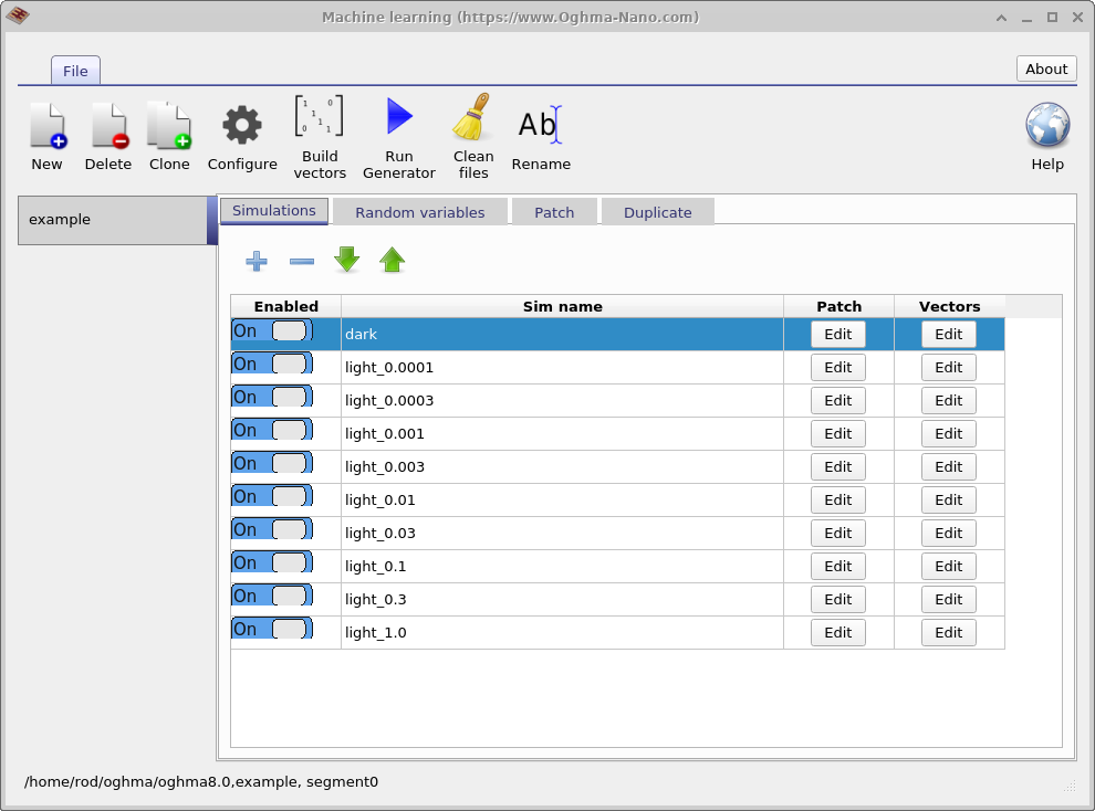
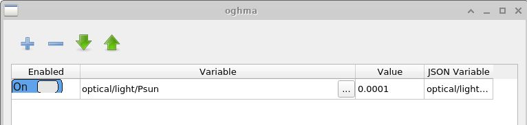
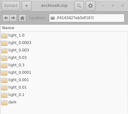
The primary purpose of this window is to generate large data sets for training machine-learning algorithms. The data set produced in this example is called example. The first tab shown is the Simulations tab, which defines the set of simulations performed for each virtual device. In this case, a dark JV curve and nine illuminated JV curves are simulated, with light intensities ranging from 0.0001 Suns to 1.0 Suns. Individual simulations can be enabled or disabled using the Enabled toggle. If the Edit button is clicked in the Patch column for the \(light\_0.0001\) entry, the Patch window shown in ?? is opened.

The purpose of the Patch window is to modify parameters within a virtual simulation. In this example, multiple JV curves are generated under different illumination conditions using the same base device structure. To achieve this, the light intensity must be adjusted independently for each simulation. Opening the patch window for \(light\_0.0001\) shows that the simulation parameter optical/light/Psun, which controls the illumination intensity, is set to \(0.0001\). For the dark simulation, the same parameter is set to \(0.0\). In this way, multiple experimental conditions can be simulated consistently using a single base simulation.

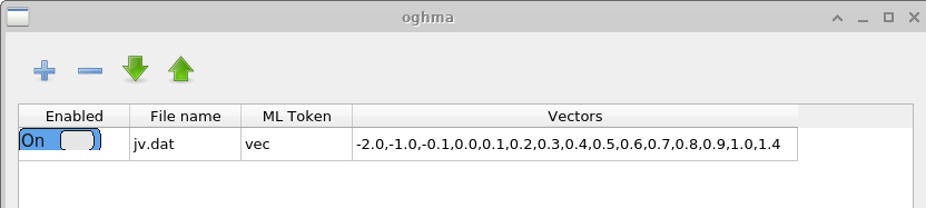
The Vectors window defines which data are extracted from the completed simulations to form the machine-learning input vectors. In this example, data points between −2.0 V and 1.4 V are extracted from the file \(jv.dat\), which contains the simulated current–voltage characteristics. For time-domain simulations, a user might instead extract data from files such as \(time\_i.csv\) or any other appropriate output file. The number of points used to construct each input vector is chosen by the user. Longer vectors increase the computational cost of training but may capture more detailed features of the JV curve.

4. Defining the random variables

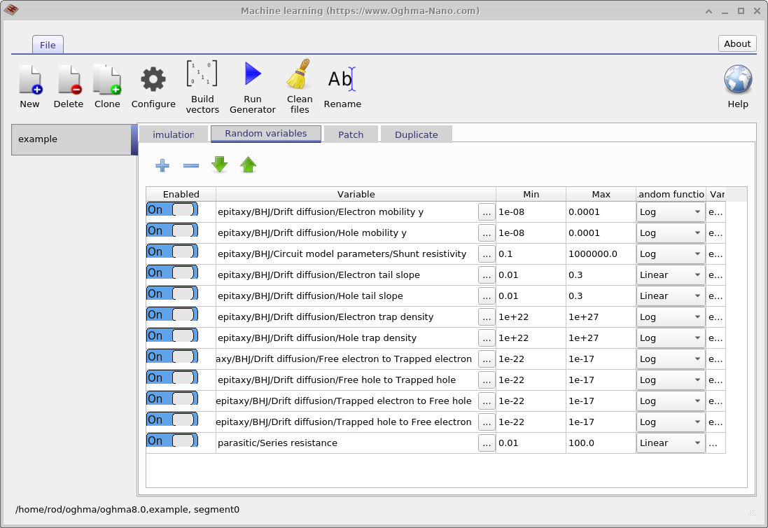
The next step is to define which model parameters are to be randomised. This is done using the Random variables tab in the main machine-learning window. The table contains five columns. The Enabled column determines whether a parameter is included in the randomisation process. The Variable column specifies which simulation parameter is varied. The Min and Max columns define the lower and upper bounds of the parameter range, and the Random function column specifies whether values are drawn from a linear or logarithmic distribution.

Logarithmic distributions are recommended for parameters that span multiple orders of magnitude, while linear distributions are appropriate for parameters that vary over a relatively narrow range. Using a logarithmic distribution ensures that values are sampled evenly when viewed on a logarithmic scale, rather than being clustered toward the upper end of the range. For example, an appropriate linear parameter would be the Urbach energy, which typically varies between 30 and 150 meV. In contrast, trap densities are well suited to logarithmic sampling, as they may vary from \(1 \times 10^{15}\,\mathrm{m^{-3}}\) to \(1 \times 10^{25}\,\mathrm{m^{-3}}\).

5. Defining the number of simulations

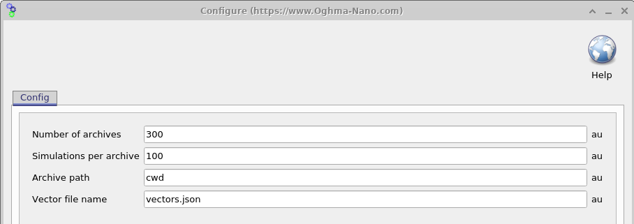
Once the simulation has been configured, the next step is to determine how many virtual devices with randomised parameters should be generated. Opening the Settings window (see 18.6) allows this to be controlled using two parameters: Simulations per archive (\(N_{\mathrm{sim}}\)) and Number of archives (\(N_{\mathrm{arc}}\)). The total number of virtual devices generated is given by \(N_{\mathrm{sim}} \times N_{\mathrm{arc}}\).

Simulation results are written to ZIP files referred to as archives, with each archive containing \(N_{\mathrm{sim}}\) virtual devices. In the example shown here, \(N_{\mathrm{sim}} \times N_{\mathrm{arc}} = 3000\) virtual devices are generated and stored across 100 archive files. It is important to note that, in this example, each virtual device consists of one dark JV simulation and nine illuminated JV simulations. As a result, the total number of output files can grow rapidly.

To manage this, data generation is performed in batches. A group of \(N_{\mathrm{sim}}\) simulations is generated and run by OghmaNano, then written to a single archive, and this process is repeated until \(N_{\mathrm{arc}}\) archives have been produced. This approach limits data loss to the archive currently being generated if the process is interrupted, and also simplifies file transfer and improves robustness against corruption. Simulation execution is parallelised across all available CPU cores, while archive creation is performed on a single core.

6. Running the data-set generator

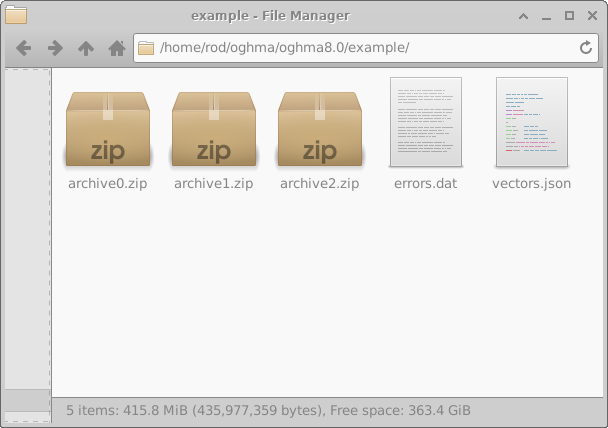
Once the configuration is complete, pressing the Run generator button in the main Machine learning window (18.2) starts the data-set generation process. OghmaNano will then begin executing the simulations defined for each virtual device. When the process has finished, a directory named example will appear in the simulation directory, as shown on the left-hand side of 18.8. For the purposes of this example, Simulations per archive was set to 10 and Number of archives was set to 3 in order to reduce run time.

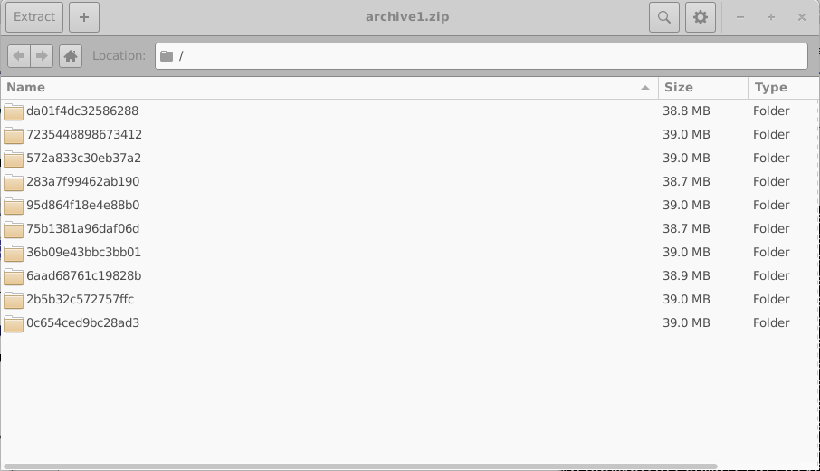
Any errors encountered during simulation are written to the file errors.dat. Opening archive0.zip reveals the internal structure of an archive, shown on the right-hand side of 18.8. Each archive contains a collection of directories, each corresponding to a single virtual device.

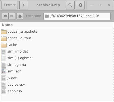
These directories are named using random 16-digit hexadecimal identifiers. Each directory contains the complete set of simulations for one virtual device; in this example, one dark JV simulation and nine illuminated JV simulations. The contents of one such directory are shown in the left-hand side of 18.10. Opening an individual simulation directory (18.10, right) reveals a full OghmaNano simulation, including the sim.json file and the jv.dat file containing the simulated current–voltage characteristics. Additional data, such as optical outputs and cache files, may also be present.

When generating large machine-learning data sets, it is strongly recommended to minimise unnecessary output, as the total disk usage can grow rapidly. This can be achieved by configuring the simulation to produce only essential output data. Data-set generation is performed in batches, with simulations executed in parallel across all available CPU cores, while archive creation is handled on a single core.

In this illustrative example, only three archives are generated. In a typical production run, however, it is common to generate on the order of 200 archives, each containing approximately 200 virtual devices.

In the above example we only have three archives but in a normal simulation run one would have up to 200 archives each with 200 simulations in each.

7. Compiling the results into a single file

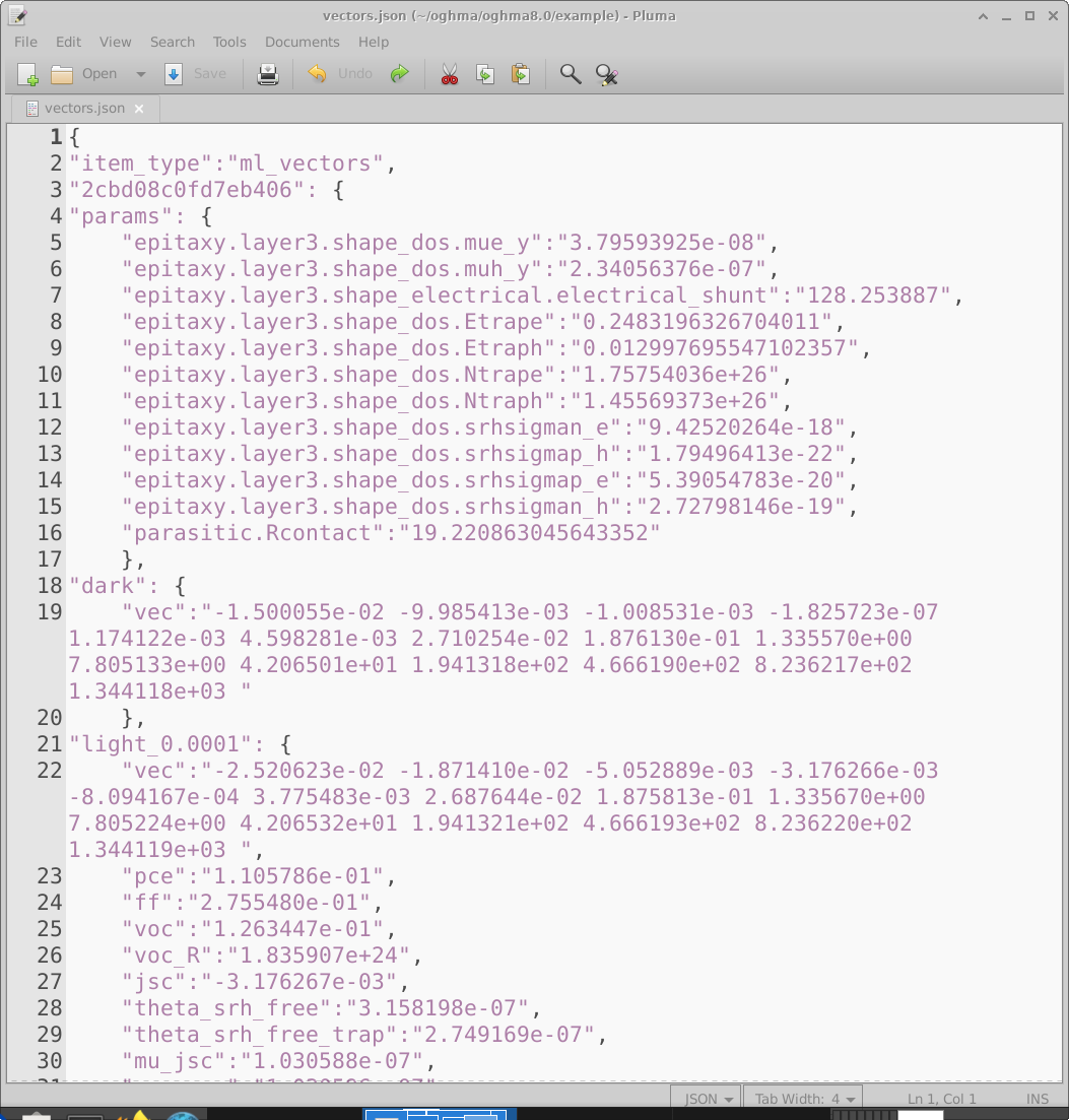
Once the simulations have completed, the raw OghmaNano output must be converted into a single vectors file suitable for training a machine-learning model. Clicking the Build vectors icon in the main Machine learning window (18.2) causes OghmaNano to open each virtual device directory, extract the requested outputs, and compile them into a single vectors.json file. An example of this file is shown in 18.11.

The vectors file is a JSON document containing all information required for supervised learning. Each virtual device appears as a separate entry. For example, the entry labelled 2cbd08c0fd7eb406 (line 3) contains, under the params section, the electrical parameters randomly selected for that virtual device. This is followed by the extracted input vectors, such as the dark JV vector (line 19) and the illuminated JV vector at 0.0001 Suns (line 22). The numerical units in each vector are inherited directly from the source file from which they are extracted. In this example the vectors are taken from jv.dat, which stores current density in \(A\,m^{-2}\) as a function of voltage, so the vector values are in \(A\,m^{-2}\). After the input vectors, additional scalar outputs (for example PCE) are stored for convenience.

There will be one entry in this file for every virtual device generated. Once vectors.json has been produced, it can be used as the training data set for the machine-learning workflow of your choice. Some users find it easier to import the data into TensorFlow after converting it to CSV; this can be done using standard Python libraries.

8. From data set to machine learning

The previous sections describe how OghmaNano is used to generate a complete machine-learning data set in JSON format. At this point, the data-generation pipeline is finished: for each virtual device, the file contains the randomly chosen model parameters together with the corresponding simulation outputs encoded as input vectors.

The next step is to import this data into a machine-learning framework of your choice. In practice, this typically involves reading the vectors.json file and converting it into a tabular format such as CSV, which can then be used for training, validation, and testing. This conversion can be performed straightforwardly using standard scripting tools (for example, Python).

Once converted, the data can be used to train a neural network or other regression model implemented using a machine-learning framework such as TensorFlow, PyTorch, or a similar library. From this point onward, the choice of network architecture, loss function, and training strategy is application-specific and independent of OghmaNano.

In this way, OghmaNano provides a complete and automated pipeline for generating physically consistent training data, leaving the subsequent machine-learning model development and optimisation entirely under the user’s control.