Materials database: Part A - Introduction
This page explains what’s in the OghmaNano Materials database, how to open and edit entries, how to import n–k or absorption data (including unit conversion), and where materials are stored on disk.
1. Overview
The OghmaNano Materials database stores a range of physical and reference properties for each material. These are organised into categories so that simulations can use consistent, centralised data. The main information includes:
- Optical constants:
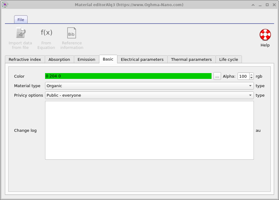
- Basic metadata: physical colour for 3D drawings, material type, privacy settings, and a change log ??.
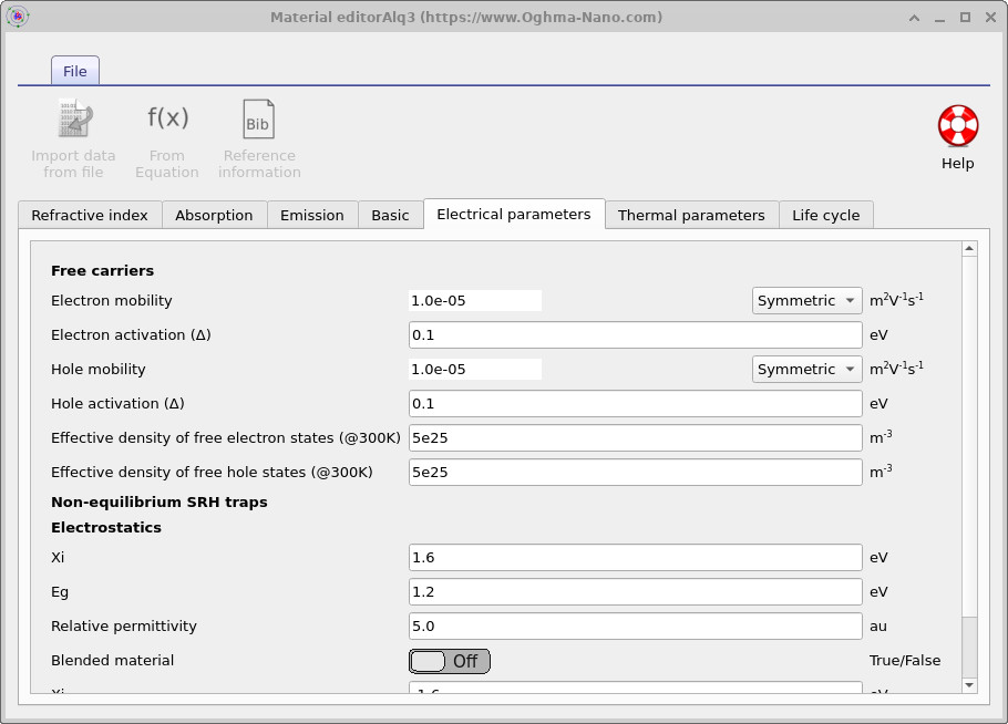
- Electrical parameters (reference only): These values do not affect simulations directly; they act as “ground truth” for restoring modified materials. The exception is band-diagram sketches: if Ec/Ev are not defined in a device, the UI falls back to these reference values ??.
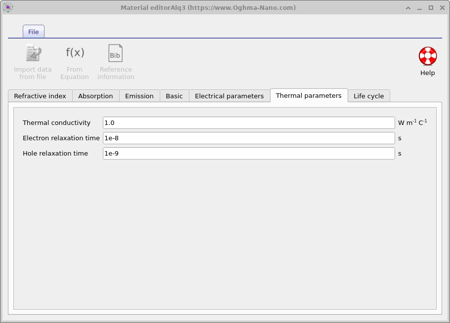
- Thermal properties: conductivity, relaxation times, and related parameters ??.
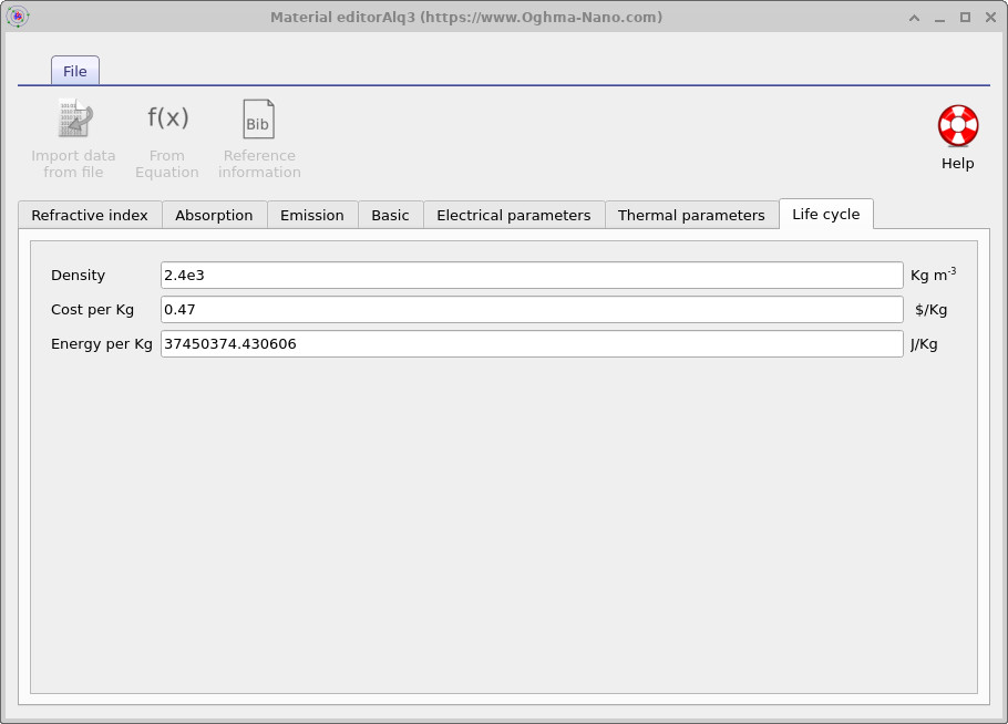
- Life-cycle data: density, cost per kilogram, and energy per kilogram for embodied-energy and cost calculations ??.
Together, these datasets provide a central, consistent definition of each material for use across all simulations.
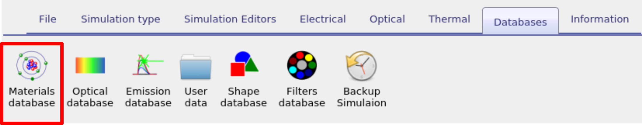
2. Accessing the materials database
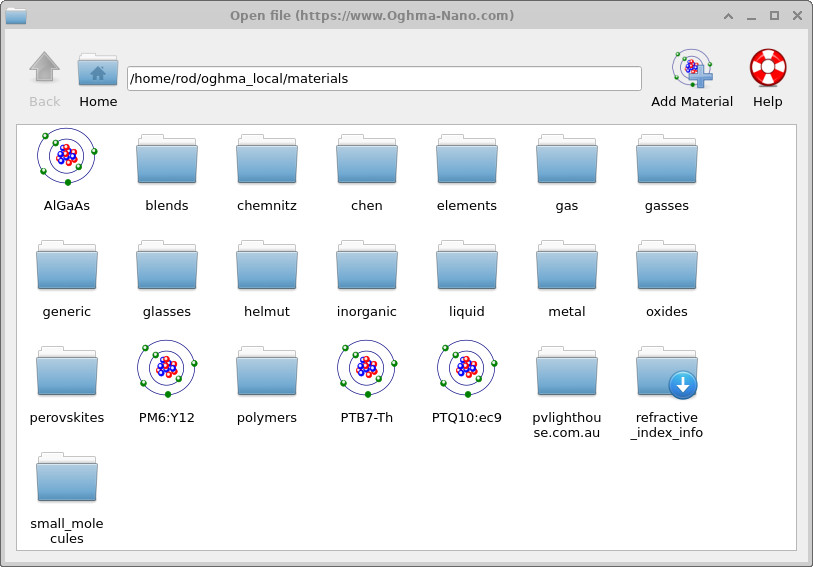
Open the Materials Database from the Databases ribbon by clicking the Materials Database icon ??. This launches the Materials Database browser ??, which shows top-level folders alongside individual materials represented by “atom” icons. Double-click a folder to explore the structured library—organised by material class (e.g., metals, oxides, glasses) and including a dedicated collection imported from refractiveindex.info. Click an atom icon to open that material’s property views described above. Use Help for guidance, and Add Material to create a new entry or import your own datasets.
3. Adding materials to the database
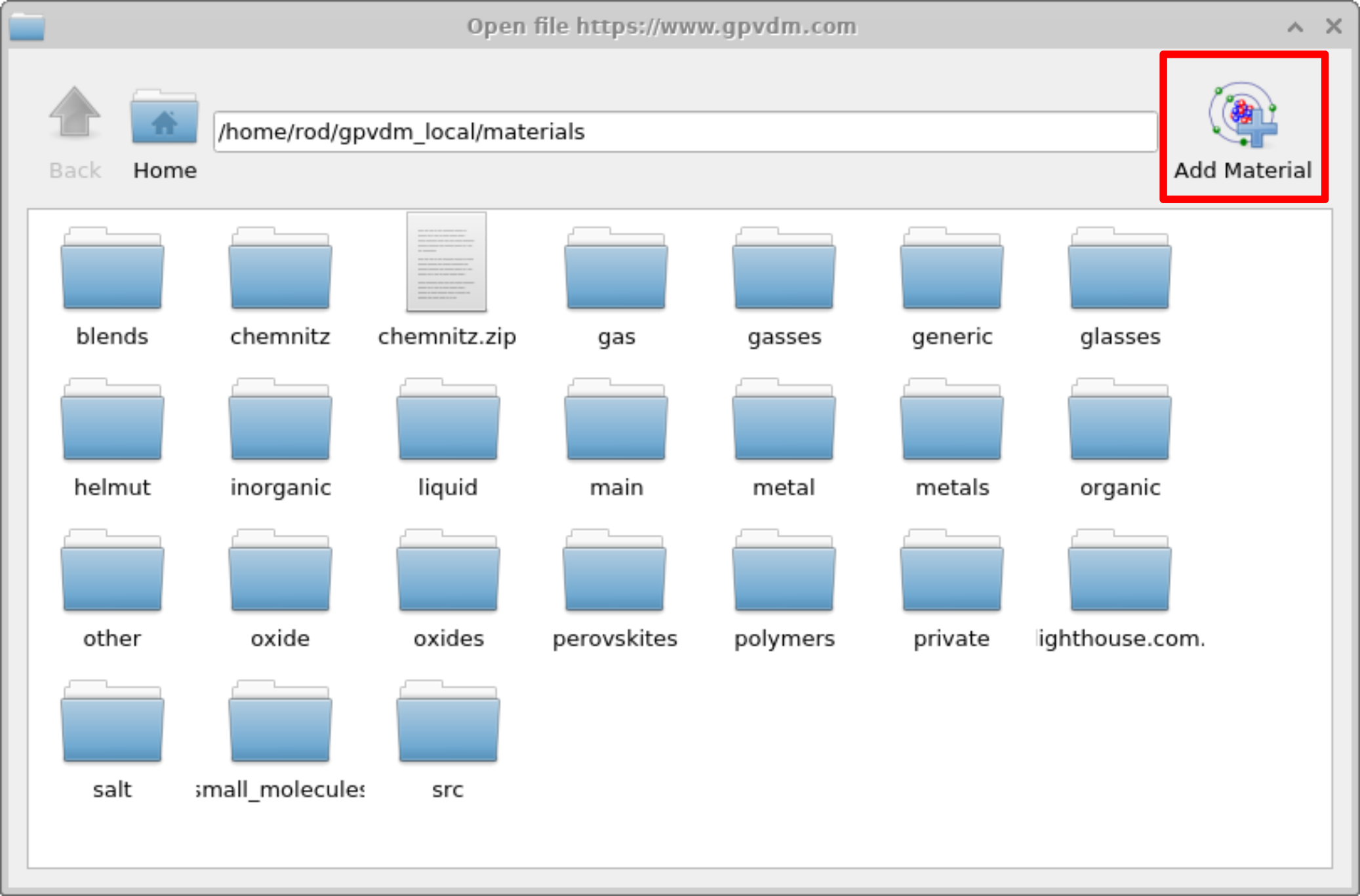
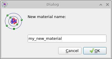
To add a new material open the Materials database, then click add material in the top right of the window (??), this will bring up a dialogue box which will ask you to give a name for your new material, this is visible in figure ??. In this case we called the material my_new_material.
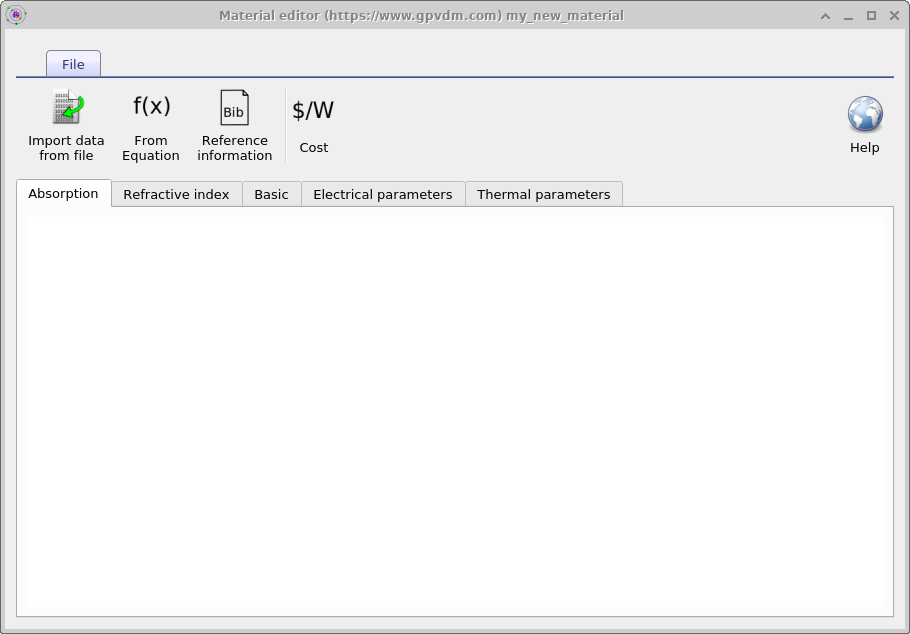
Once you have clicked OK the new material will appear see Figure [fig:materialadd4], open it by double clicking on it. This will bring up an empty material window with no data. See Figure [fig:materialadd5].
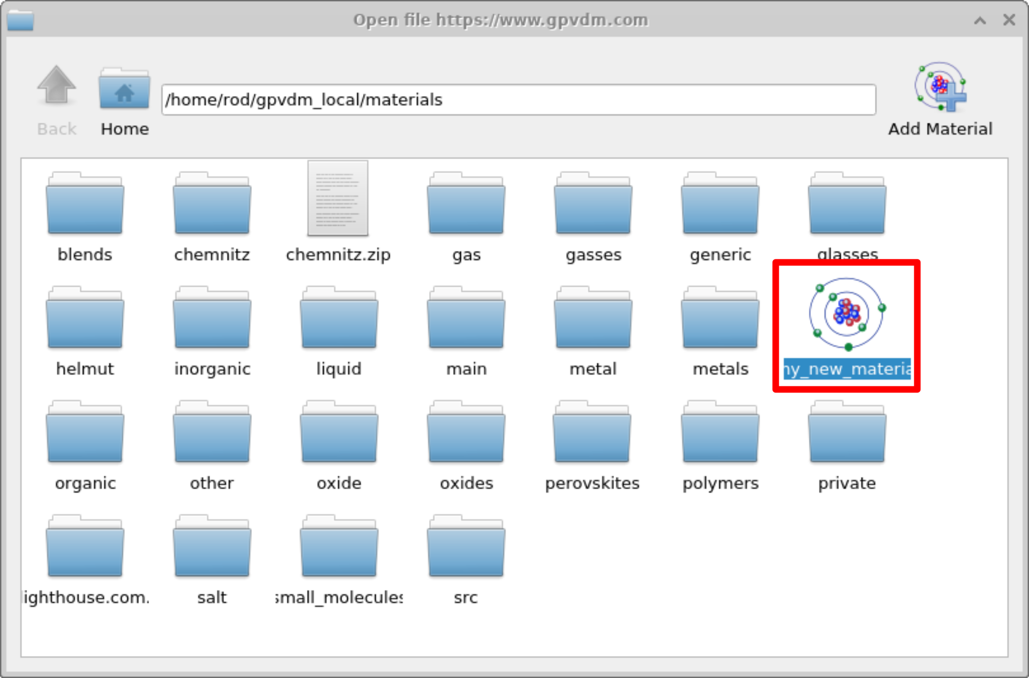
my_new_material added to the Materials database.
my_new_material, initially empty of data.
4. Understanding n/k data (n/alpha data)
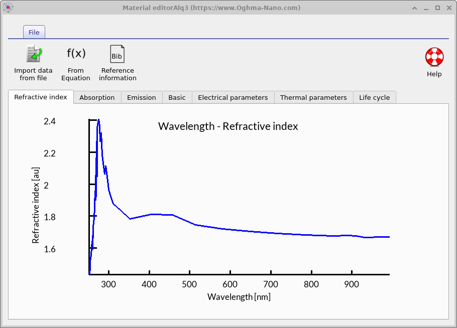
Before try to add n/k (n/alpha data) to OghmaNano , it’s important to understand what n–k data is. n–k data describes the complex refractive index of a material: the real part n and the imaginary part k.
- n (real refractive index): governs how light bends when entering the material (e.g. the beam deviation you see with a prism).
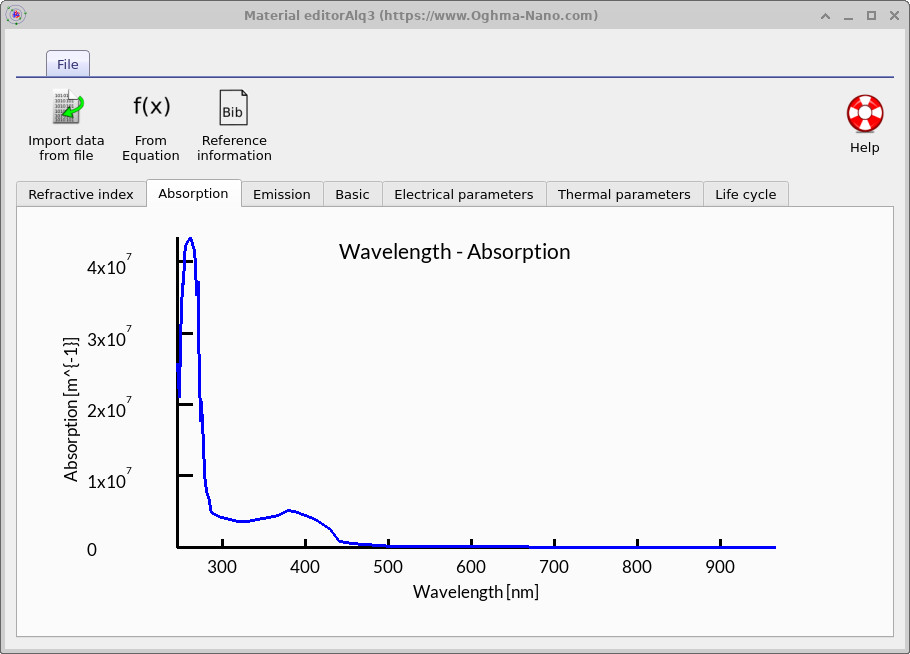
- k (extinction coefficient): governs optical loss due to absorption. A material with high k absorbs strongly (e.g. muddy water); a material with low k absorbs weakly (e.g. clear water).
There are several ways you will see optical loss written in the literature. Common forms include the absorption coefficient α (loss per metre, units m−1), the extinction coefficient k (the imaginary part of the refractive index, dimensionless), and absorbance (also called optical density), which is a logarithmic measure of transmission typically used in spectroscopy. It’s important to note that these are all the same physical quantity in principle, just expressed in different forms. OghmaNano accepts the absorption coefficient α in units of m−1. The box below explains the differences between these quantities and how to convert between them.
n, k, and absorption α — at a glance
The complex refractive index is \( N(\lambda) = n(\lambda) + i\,k(\lambda) \), where \(n\) (refractive index) and \(k\) (extinction coefficient) are dimensionless. OghmaNano stores:
- n(λ) in
n.csv(dimensionless) - α(λ) — absorption coefficient — in
alpha.csv(\(\mathrm{m^{-1}}\))
If you have \(k(\lambda)\) instead of \( \alpha(\lambda) \), the importer converts using: \( \displaystyle \alpha(\lambda) = \frac{4\pi\,k(\lambda)}{\lambda} \) (with \( \lambda \) in metres → \( \alpha \) in \( \mathrm{m^{-1}} \)).
From absorbance/optical density (A) or transmittance (T)
- \( A = -\log_{10}(T) \)
- \( \displaystyle \alpha = (\ln 10)\,\frac{A}{d} \) where \( d \) is film thickness (m)
Units to use: \( \lambda \) in metres (m); \(n\) and \(k\) are dimensionless; \( \alpha \) in \( \mathrm{m^{-1}} \). Curves labelled “a.u.” for absorption cannot be used directly.
Worked example — convert \(k \rightarrow \alpha\)
Given \( k=0.02 \) at \( \lambda=500\,\mathrm{nm}=5.00\times10^{-7}\,\mathrm{m} \):
\( \displaystyle \alpha = \frac{4\pi k}{\lambda} = \frac{4\pi \times 0.02}{5.00\times10^{-7}} \approx 5.03\times10^{5}\ \mathrm{m^{-1}} \).
5. Importing n/alpha data (or n/k data)
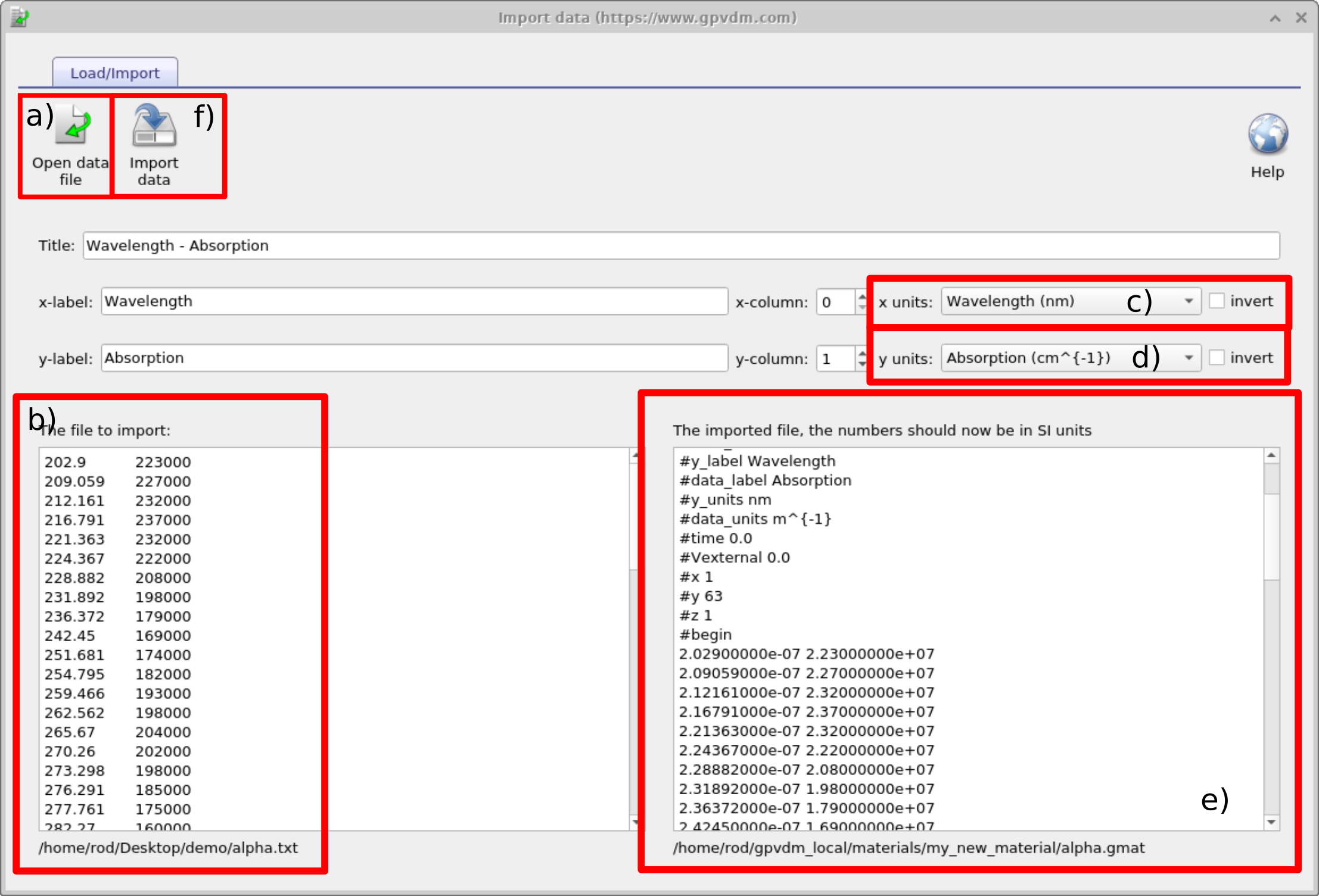
Click Import data from file at the top-left of the material window ?? to open the Import Data wizard ??. If you have the Refractive Index tab open, when you click Import Data from File, the data will be imported into the refractive index dataset. If you have the Absorption tab selected, it will be imported into the absorption dataset. Make sure you import the right data into the right tab. The wizard loads your file, maps its columns, and converts units to the format OghmaNano uses.
Expected file formats (two columns, SI):
- Refractive index n(λ): wavelength (m) vs refractive index (dimensionless).
- Absorption α(λ): wavelength (m) vs absorption coefficient (m−1).
If your source uses other units (e.g. nm, μm, cm−1, or eV for photon energy), the wizard converts them (e.g. nm → m, cm−1 → m−1, eV → m via λ = hc/E). If your file has k(λ), the wizard can also compute absorption using α(λ) = 4πk(λ)/λ.
Workflow:
- Open your text/CSV file.
- Check the preview (left panel).
- Select the x-axis units (wavelength) and the y-axis quantity (n, k, or α) and units. These need to match the units on your input data For k choose ""
- Review the converted SI data (right panel).
- Click Import data to save it to the material.
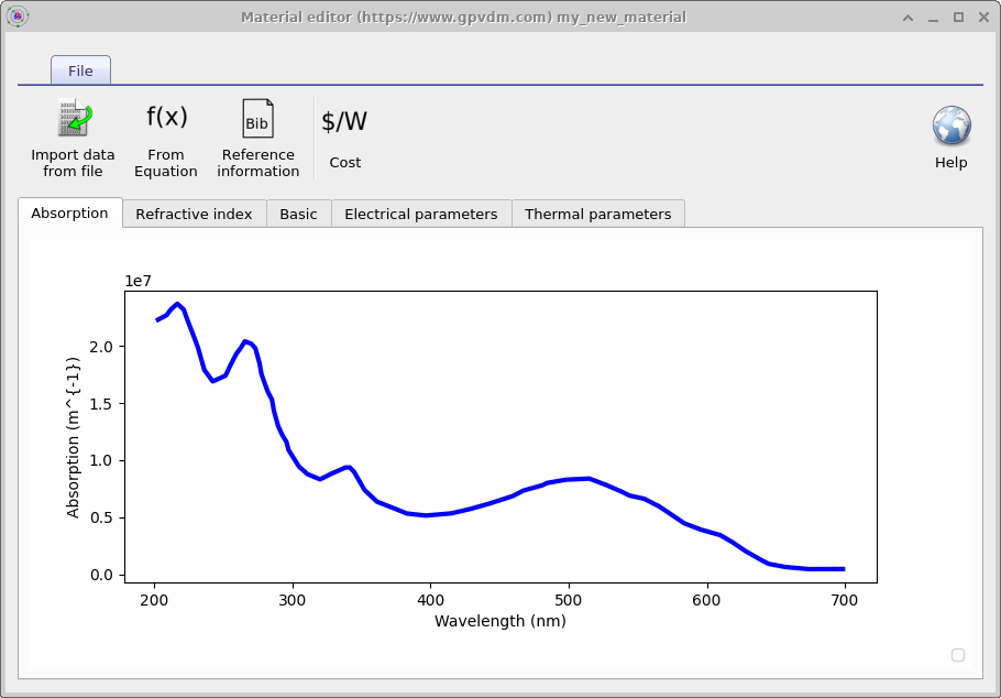
The wizard view is shown in ??; after import, the plots update in the material editor ??. If you import only absorption, remember to also provide refractive index before using the material in a simulation.
Common pitfalls
- Absorption in “a.u.” or normalised to 1 → not usable, as it has lost its magnitude information..
- The final imported values will be in SI units, look at them - do they make sense - do a ballpark magnitude check?
👉 Next step: Now continue to Part B for tips on finding n/k data for your material system.