Optical Spectra Database

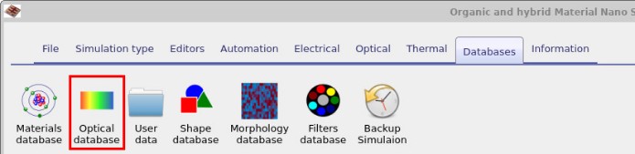
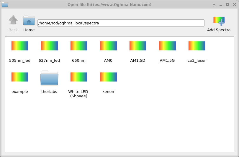
Click the Optical Database icon in ?? to open the optical database, which stores optical spectra such as laser profiles, measured solar spectra, and other experimental datasets. The database view is shown in ??.

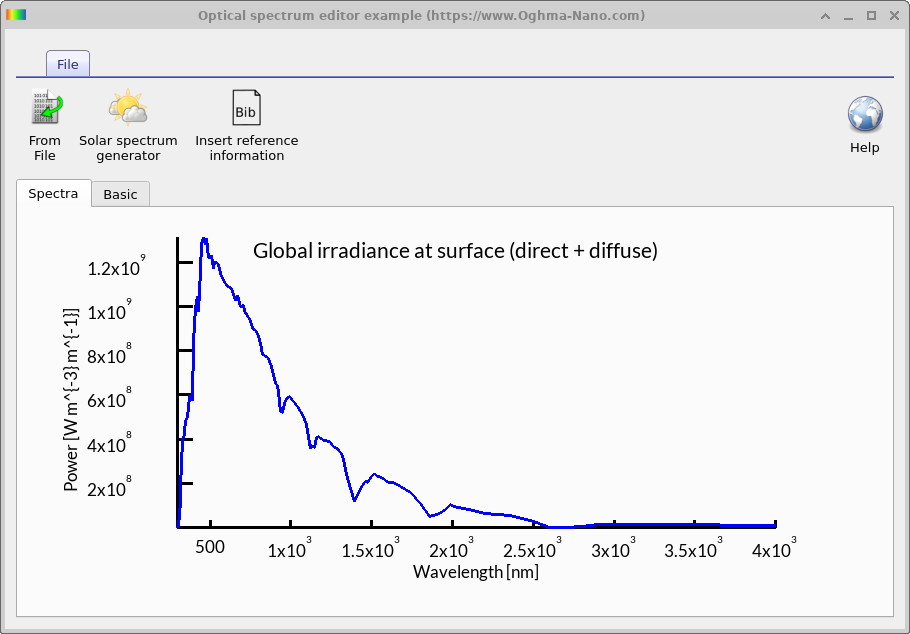
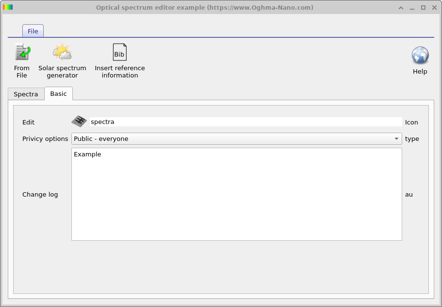
OghmaNano Databases ribbon with the Optical database icon highlighted. — The *Databases* ribbon in OghmaNano. Selecting the **Optical database** opens the optical spectra database.

OghmaNano window showing the Optical database directory with available spectra entries. — The *Optical database* directory, listing available spectra. Double-clicking an entry opens its data in the editor.

Double-clicking a spectrum opens it in the Optical Spectrum Editor (??), where you can view existing data or import new spectra. The Basic tab (??) provides fields for notes, metadata, and privacy options.

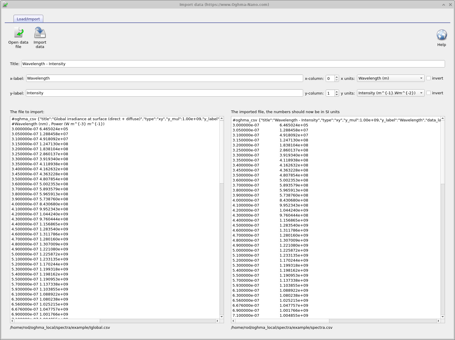
To import data, click From File in the editor to open the import window (??). Load your raw file with Open data file (shown in the left panel), then choose the correct units for each column (e.g., nanometers for wavelength). The tool automatically converts the data into SI units (right panel). Clicking Import data adds the converted spectrum to the Optical Spectrum Editor.

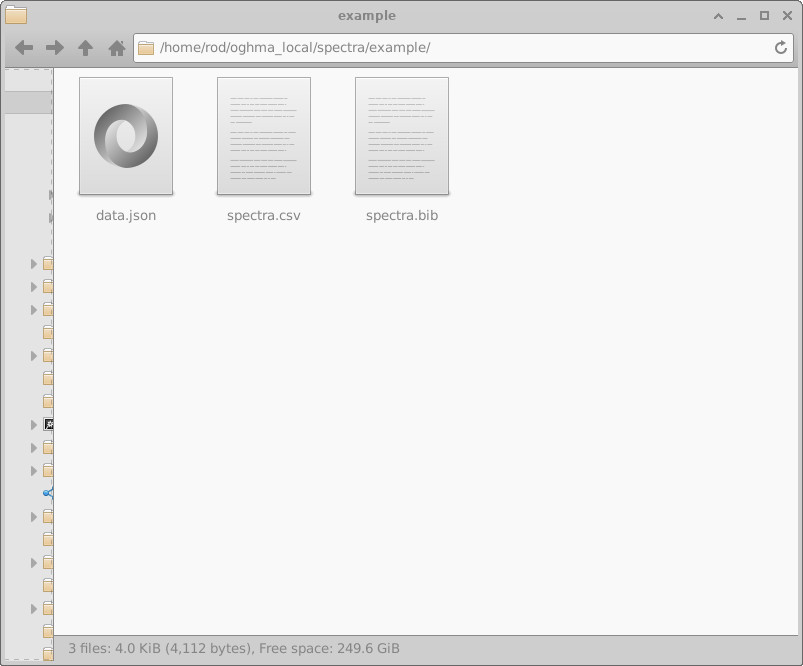
OghmaNano optical spectrum editor showing a solar spectrum plot of global irradiance versus wavelength. — The *Spectra* tab in the Optical Spectrum Editor. Here, a solar spectrum is displayed as *Power vs. Wavelength*.

OghmaNano optical spectrum editor showing the Basic tab with metadata fields including privacy options and description. — The *Basic* tab of the Optical Spectrum Editor. Use it to add notes, set privacy, and provide descriptive metadata for the spectrum.

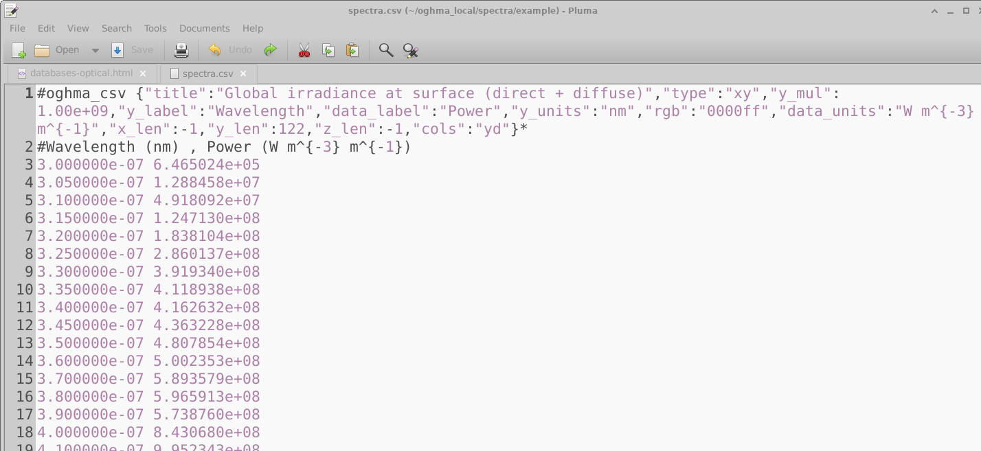
Spectra are saved in your local database folder (??) under oghma_local/spectra/<entry>/. Each entry contains a data.json file, a spectra.csv file with numerical data, and optionally a spectra.bib reference file. Opening spectra.csv (??) shows a header followed by wavelength (m) and spectral irradiance (W m⁻³). All spectra are stored in SI units. By definition, the integral of each spectrum gives the total power density (W m⁻²), and this must be correct because the simulator does not renormalize imported data. If in doubt, write a small script to integrate the spectrum and confirm the power density. For a standard solar spectrum (AM1.5G), this should be approximately 1000 W m⁻².

Windows: quickly open your local spectra folder

Press Win+R, type %USERPROFILE%\oghma_local\spectra, and press Enter.
Each spectrum is stored in its own subfolder (e.g., ...\spectra\example\).

OghmaNano data import window showing wavelength–intensity data being mapped to SI units. — The *Data Import* window. Raw input values (left) are mapped to axes and units. The converted values (right) are always in SI units, ready for the model.

File browser window showing the Oghma local spectra directory with JSON, CSV, and bibliography files. — Example spectra entry stored in `oghma_local/spectra`. Each entry contains JSON metadata, a CSV with spectral data, and optionally a bibliography file.

Text editor window displaying the contents of spectra.csv with a header and wavelength–power values in SI units. — The contents of `spectra.csv`. Columns list wavelength in meters and spectral irradiance in W m⁻³, always in SI units.

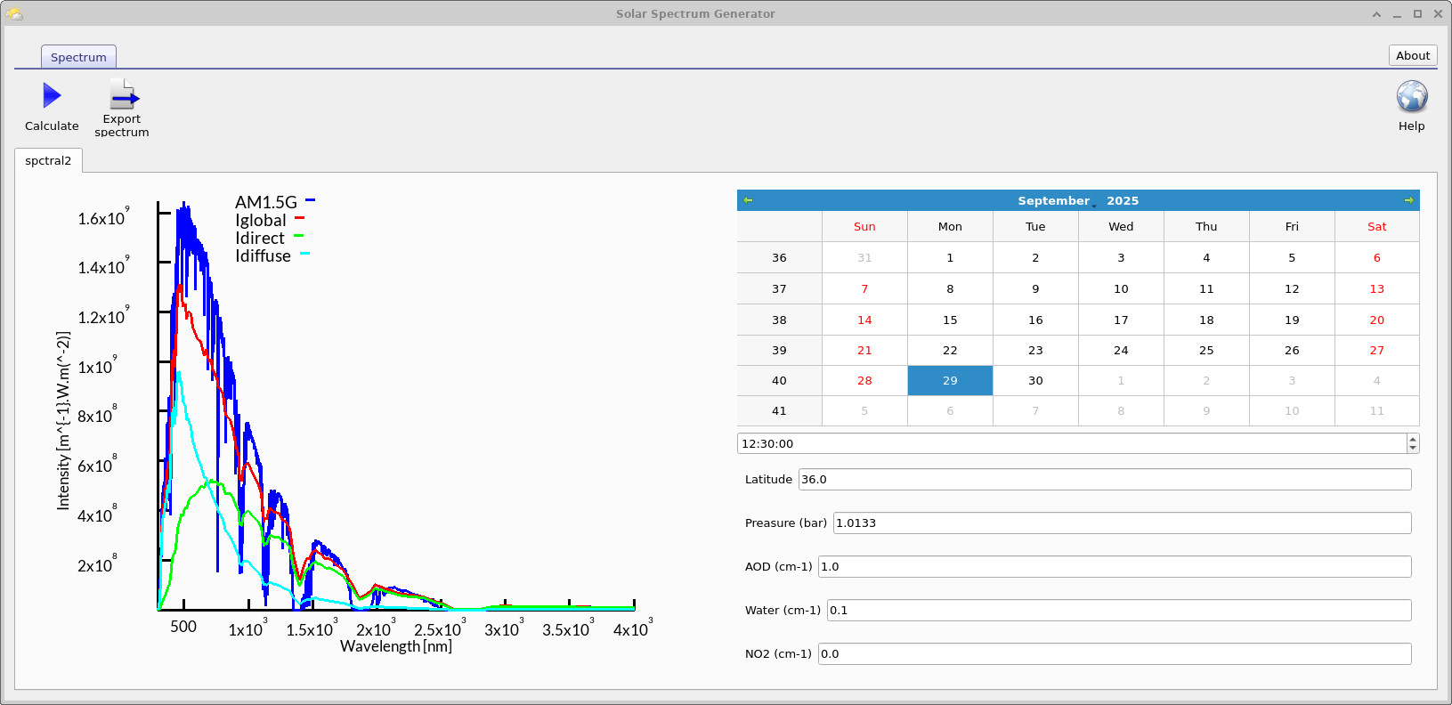
Solar Spectrum Generator

The Solar Spectrum Generator (??) can be launched from the Optical Spectrum Editor. It compares the AM1.5G reference spectrum with calculated I_global, I_direct, and I_diffuse components, and allows spectra to be generated for different times of day, geographic locations, and atmospheric conditions (pressure, water vapour, and aerosol loading).

The generator is based on the Simple Solar Spectral Model for Direct and Diffuse Irradiance on Horizontal and Tilted Planes at the Earth's Surface for Cloudless Atmospheres by Bird and Riordan (1986), published in the Journal of Applied Meteorology and Climatology. You can view the original paper here. This semi-empirical model computes solar spectral irradiance at the Earth’s surface by accounting for key atmospheric processes such as Rayleigh scattering, ozone absorption, uniformly mixed gases, water vapour absorption, and aerosol extinction. With inputs including location, time of day, altitude, and atmospheric parameters, the model partitions the solar spectrum into global, direct, and diffuse components. The AM1.5G reference is provided as a benchmark, enabling users to generate site- and condition-specific spectra that reflect both geometric factors (solar zenith angle, air mass) and atmospheric properties (pressure, water vapour, and aerosol optical depth).

OghmaNano Solar Spectrum Generator window showing AM1.5G reference spectrum compared with calculated global, direct, and diffuse components. — The *Solar Spectrum Generator* window. Compare the AM1.5G reference spectrum with calculated components (*I_global*, *I_direct*, *I_diffuse*), and regenerate spectra under different conditions.