FDTD in OghmaNano
1. Introduction
The Finite-Difference Time-Domain (FDTD) method is one of the most widely used techniques in computational electromagnetics. It works by discretising both space and time, then numerically integrating Maxwell’s equations step by step to follow the evolution of the electromagnetic field. Because no simplifying assumptions are made about geometry, materials, or the form of the solution, FDTD can handle arbitrary device structures, complex boundaries, and strongly scattering or resonant systems. This makes it a powerful tool for studying nanophotonic devices, photonic crystals, plasmonic structures, and waveguides, as well as for visualising how fields propagate and interact in real space and time. However, this generality comes at a cost: FDTD is computationally intensive, requiring large amounts of memory and many time steps per wavelength to reach a solution. Only with the growth of modern computing power has it become feasible to apply FDTD to realistic device problems.
Before choosing FDTD, it is important to consider whether it is the right tool for your problem. In many cases, using FDTD can be like using a sledgehammer to crack a nut. For example, one could model a conventional solar cell using FDTD by launching a wavefront through the top contact, simulating its evolution over thousands of time steps until steady state is reached, and then calculating absorption. However, in most device studies we are not concerned with the detailed time evolution of the optical field—sunlight varies extremely slowly—and steady-state methods such as the transfer matrix model (see Part A) are usually far more efficient.
Nevertheless, FDTD is an important and versatile method, particularly for analysing and designing complex photonic structures. It excels in cases where interference, scattering, or non-trivial geometries play a key role—for example, in photonic crystals, waveguides, and microstructured devices.
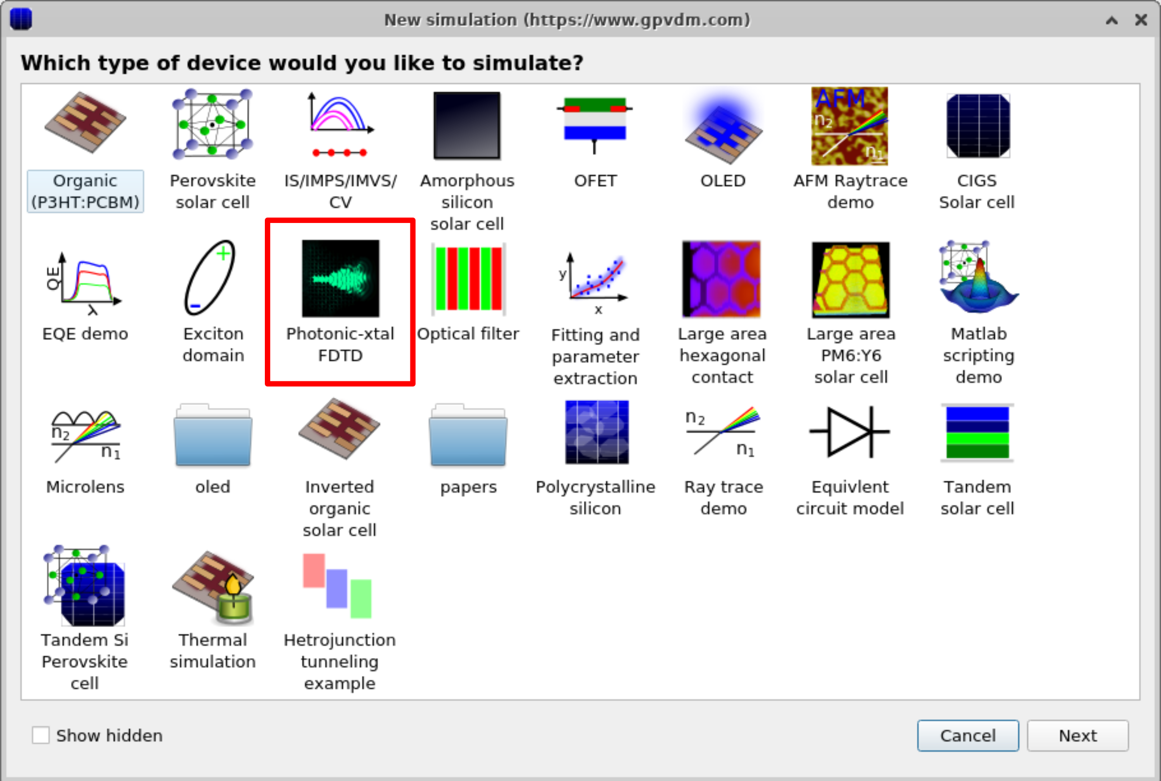
To start an FDTD simulation in OghmaNano, open the New simulation window (??) and select the Photonic-crystal FDTD demo. This will launch the initial FDTD simulation window (??), where you can explore the evolution of the optical fields in the time domain and choose which field components to display.
2. Running an FDTD simulation
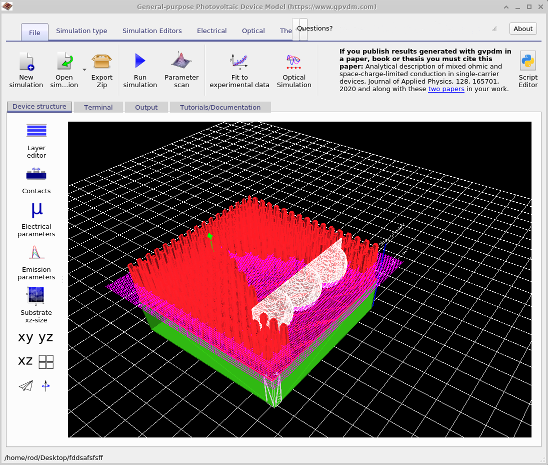
Once opened, the simulation window will look like ??. Click the Play button to start the solver. A small demo will typically run in around 30 seconds, though more complex structures may take considerably longer.
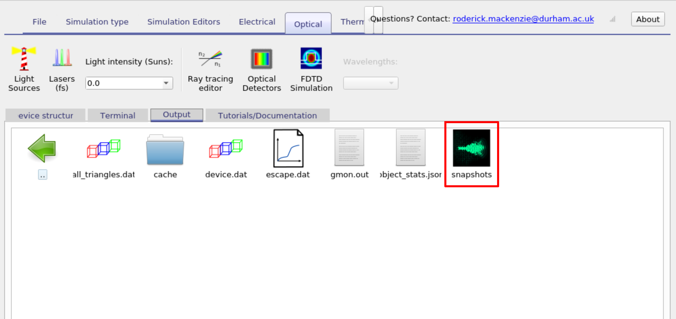
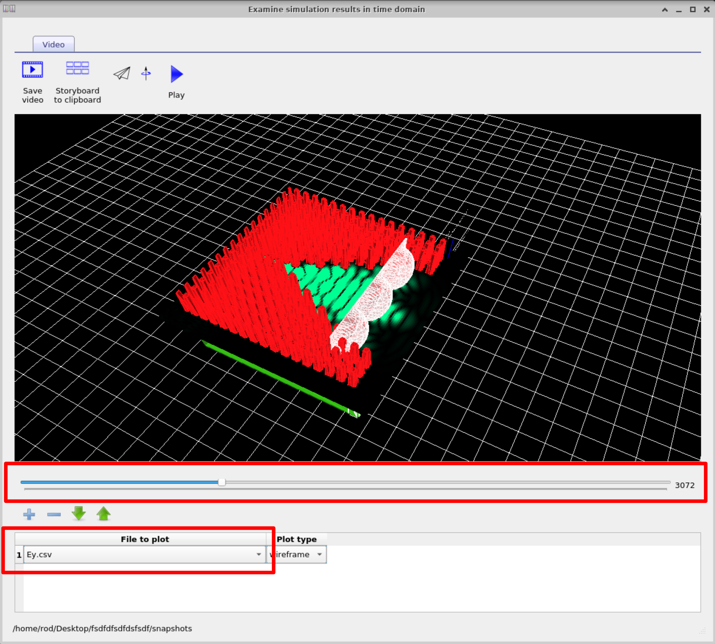
After the simulation completes, switch to the Output tab. There you will find the snapshots folder (??). Double-clicking this folder opens the FDTD snapshots window (??). This tool allows you to step through the field evolution frame by frame. Use the File to plot drop-down menu to choose which field component to display (Ex, Ey, or Ez). In this example, select Ey, then use the slider bar to explore how the field evolves over time. You can also play the animation directly or export frames as a video for presentations and publications.
3. Manipulating objects in OghmaNano
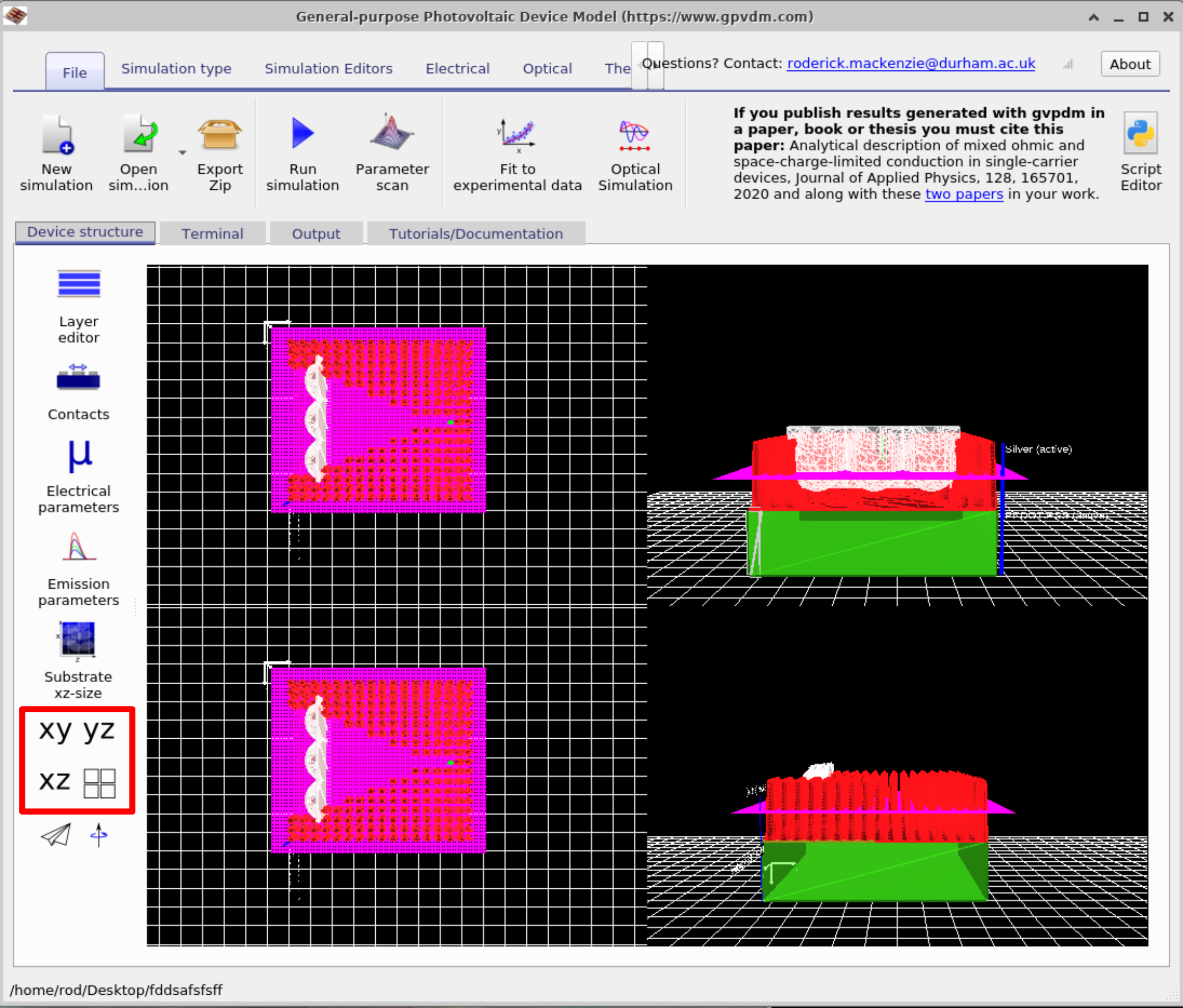
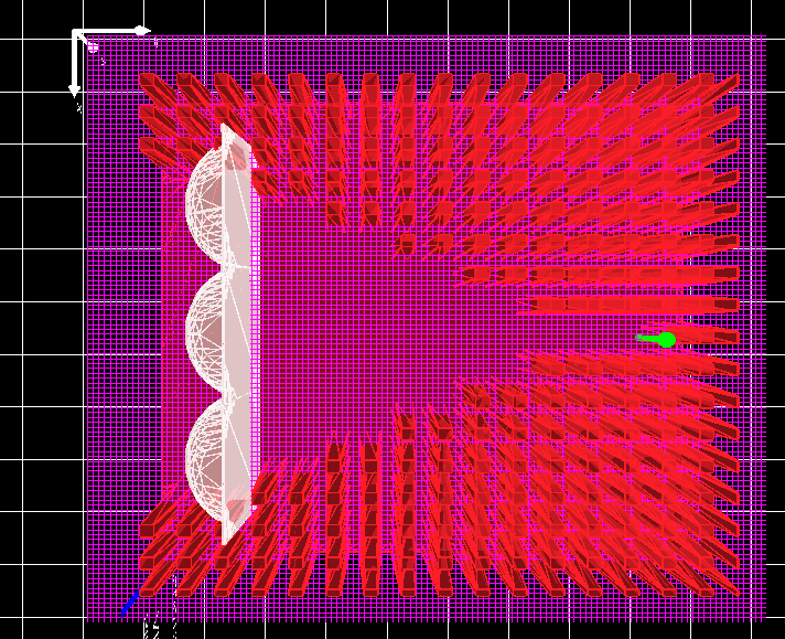
Close the snapshot viewer and return to the main simulation window. Select the Device tab. On the left-hand side you will see four view buttons: xy, yz, xz, and a grid of small square boxes (??). Try clicking each of them to explore how the device view changes. For the next steps, select the xz view so that your screen resembles the left-hand side of ??.
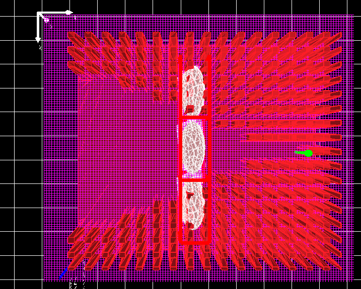
If you left-click on the lenses, you can move them around within the device. Try repositioning the lenses so that your design matches the right-hand side of ??. Holding the Shift key while dragging allows you to rotate objects in place.
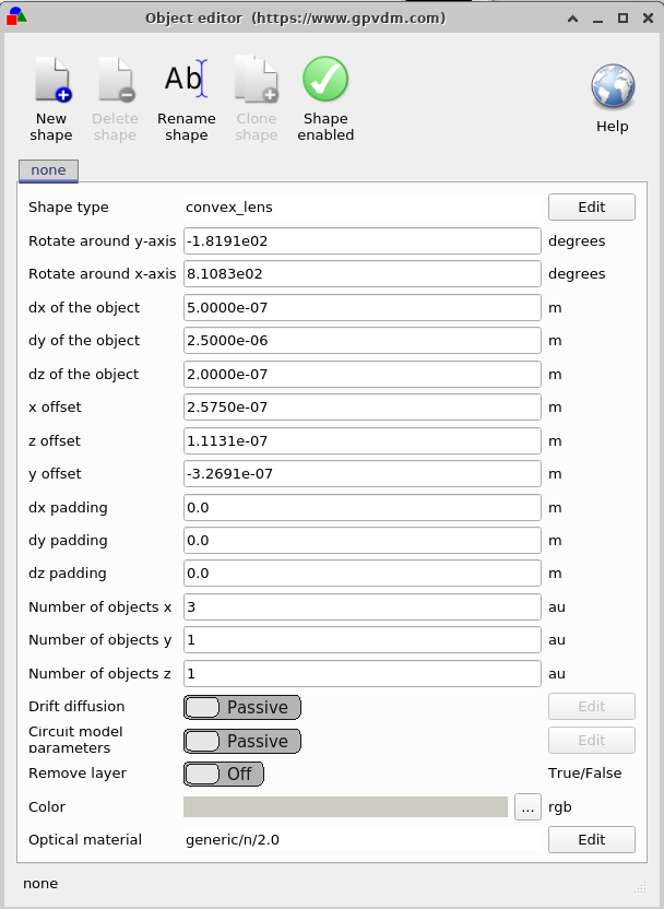
Right-clicking on a lens and selecting Edit opens the Object Editor
(??).
This editor provides full control over an object’s properties.
For example, you can change the type from convex_lens to concave_lens,
adjust its material for FDTD simulations, modify its colour, position, or rotation angle,
and re-run the simulation to see the effect.
The editor also includes a shape enabled toggle, which lets you temporarily disable an object.
If the object is electrically active, this window can also be used to configure its electrical parameters.
For advanced use, you can add your own custom shapes to the shape database.
4. Configuring the FDTD solver
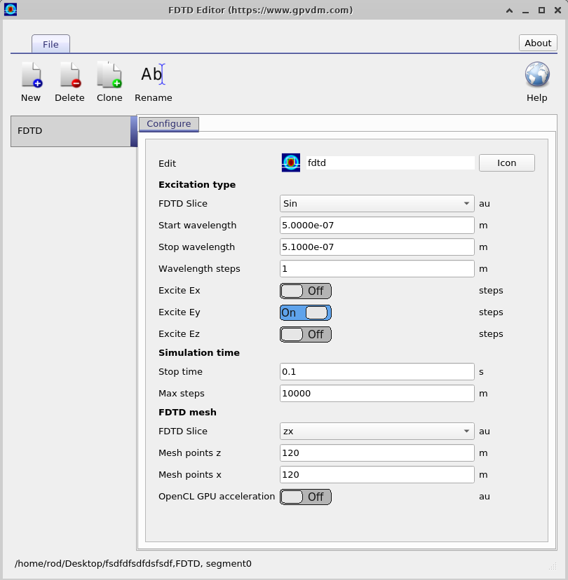
To configure an FDTD run, click FDTD Simulation on the Optical ribbon (??). This opens the FDTD Editor (??), where you control the simulation setup:
- Excitation: choose the source type (e.g., sine), select which field components to excite (Ex, Ey, Ez), and set the wavelength range and step.
- Simulation time: set the stop time and maximum time steps.
- FDTD mesh: pick the slice (xy/xz/yz) and the number of mesh points per axis; optionally enable GPU acceleration.
Adjust these parameters to match your device and accuracy/speed trade-offs, then run the solver from the main window.
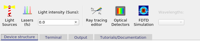
Manipulating light sources in OghmaNano
In the FDTD simulation window, the light source is represented by a green arrow (see figure ??). You can reposition this source by clicking and dragging the arrow within the device structure. Moving the arrow changes the origin point of the emitted light, which directly affects how the electromagnetic wave enters and interacts with the device.
This element corresponds to an FDTD light source. For further details on the different types of sources and their configuration, see the light source documentation.