200 mm Prime Lens Tutorial (Part B): Ray Anatomy and Vignetting Checks
1. Introduction
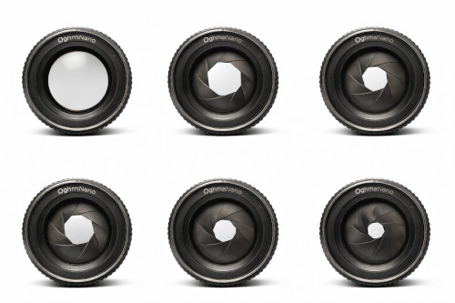
A camera lens controls how much light enters the optical system using an aperture (also called the aperture stop), a variable opening formed by overlapping metal blades. Figure (??) shows a photographic-style aperture at several settings, from fully open to nearly closed. As the aperture closes, the opening becomes smaller and its shape is increasingly defined by the blade geometry. This directly affects which rays are allowed to pass through the lens and reach the detector.
Opening the aperture wide allows more light to enter the optical system, producing a brighter image. However, in this configuration many rays pass through the outer regions of the lens, where aberrations are typically strongest, leading to increased distortion and reduced sharpness. Stopping down the aperture restricts rays to the central part of the lens, which generally produces a sharper image, but at the cost of reduced brightness. In practice, this creates a trade-off between a bright image with lower sharpness and a darker image with improved clarity.
In this part we build a practical pre-metric workflow, using only the 3D ray paths and the detector image, to answer three questions by eye: (i) where the stop is and which rays it admits, (ii) how paraxial (chief) rays differ from marginal rays, and (iii) whether clipping or vignetting is present that will compromise off-axis performance.
2. Find the stop and confirm it is open
In the 3D view, locate the stop/aperture object (typically a plate with a circular opening). Rotate the scene so you can see rays approaching and passing through the stop (??). This stop is the quickest place to understand how much light the lens can actually deliver to the image. Although all optical elements before the stop are illuminated, only rays that pass through the aperture stop are allowed to propagate through the rest of the system and reach the detector. In optical terms, the stop defines the system’s entrance pupil and therefore its numerical aperture.
d0 until you can see the stop start to clip the beam (a good “by eye”
setting is where you reject roughly half the rays for an edge-of-pupil test).
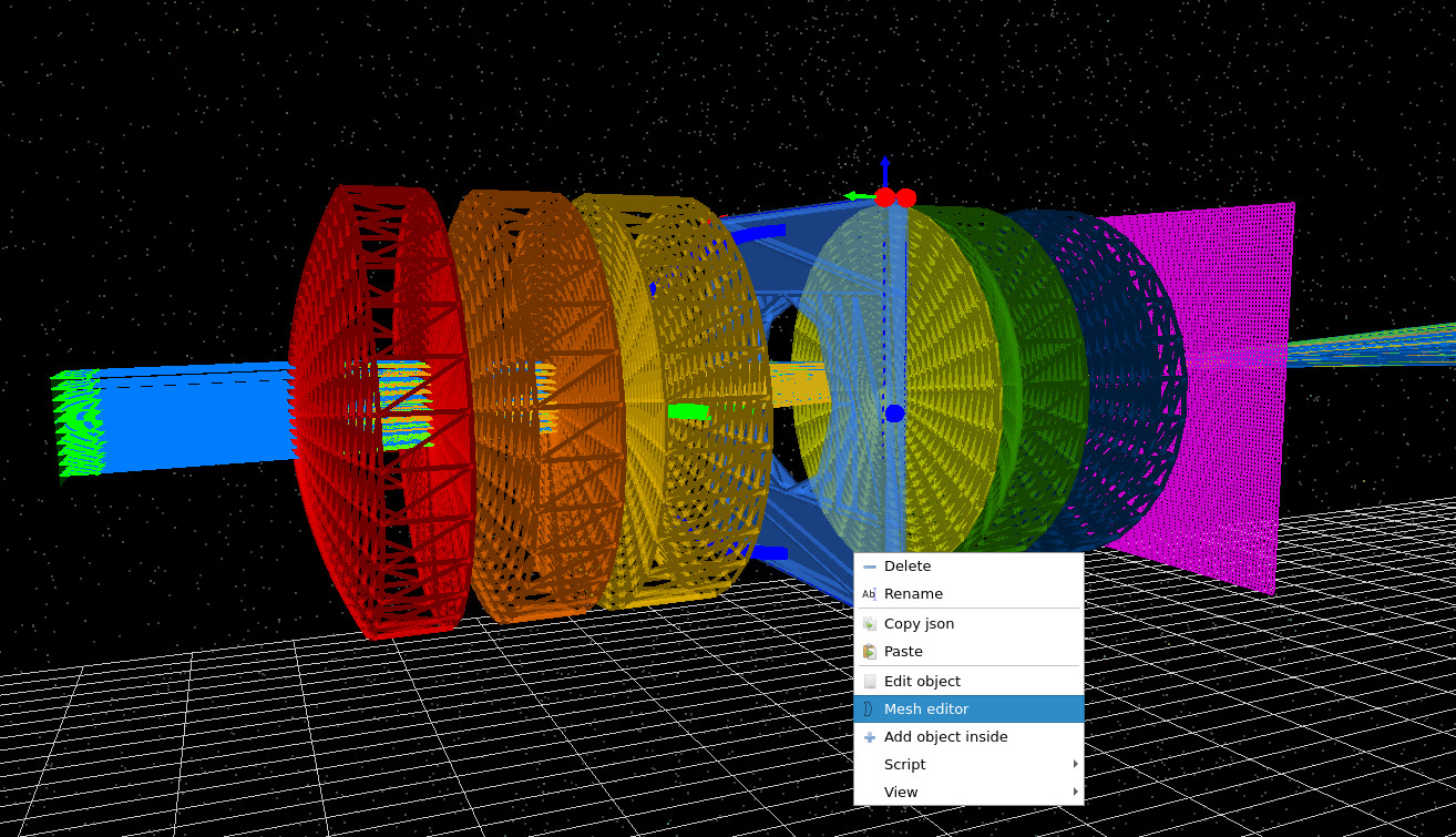
If the stop is currently closed so that no light can pass through, right-click on the stop object
and select Mesh editor
(??).
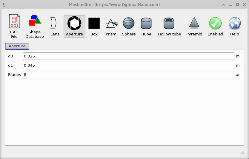
This opens the aperture mesh editor shown in the figure. In this editor, the parameter d0 controls the diameter of the clear opening.
Increasing d0 enlarges the hole and allows more rays to pass; decreasing it stops the system down.
As a practical starting point, set d0 to a value of about 0.035,
or just below the value of d1, which defines the outer radius of the square aperture.
Checkpoint
- You should be able to identify which physical object is acting as the aperture stop, even if it is not labelled as such in the model.
- You should be able to explain why rays that pass through earlier lenses may still be rejected further downstream.
- You should be able to point to the stop and say: “This single object defines the accepted ray cone for the entire system.”
2. Compare paraxial, chief, and marginal ray bundles
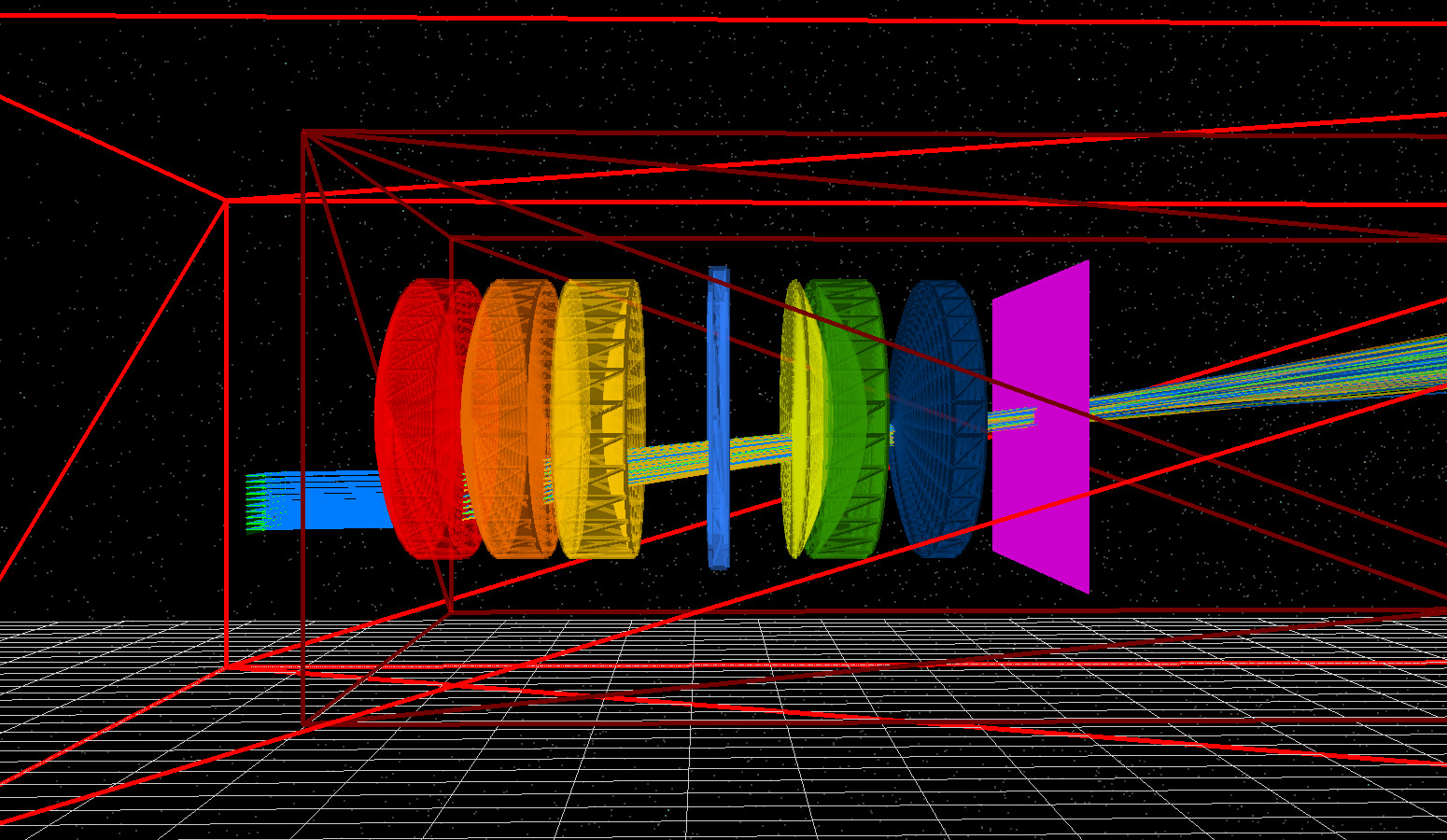
The fastest way to "read" a lens is to compare how light behaves when going through the centre of the lens (a near-axis bundle) to how light behaves when it enters the system near the edge of the lens. In optics language we are comparing the paraxial (or chief-ray behaviour) against an edge-of-pupil bundle (or marginal-ray behaviour). Generally, rays that pass close to the centre of the lens (close to the optical axis) are less distorted than rays that enter through the edge of the lens. This is because rays that enter near the edge of the lens have to be bent more to bring them onto the optical axis. You will do two runs that differ only in where the beam enters the front of the lens. Start with the baseline on-axis case: place the beam in the centre of the simulation window and click run. The light should pass cleanly through the system and form a compact footprint on the detector (??). In classical optics language, this near-axis bundle represents chief-ray (paraxial) behaviour.
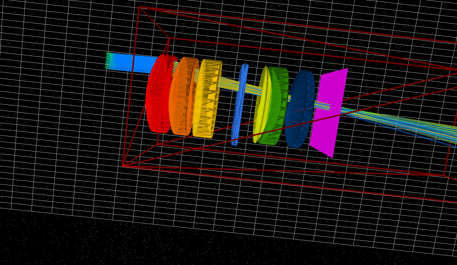
Next, translate the source so the beam enters near the edge of the first element, without changing the beam direction. This is called the marginal case, where the rays enter near the edge of the pupil. In this tutorial, you use two views of the same idea: a side view (??) and a top view (??).
These marginal rays pass near the edge of the pupil (far from the center of the optical axis) and therefore sample the most strongly aberrated regions of the optics. You are not trying to be textbook perfect here - you are simply forcing the model to show you how different ray families behave. After each run, open detector0/RAY_image.csv and compare the footprints. The central (chief-ray) bundle should typically appear compact and symmetric, while marginal rays are where asymmetry, smear, and clipping usually appear first.
3. Diagnose clipping and vignetting by eye
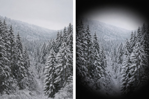
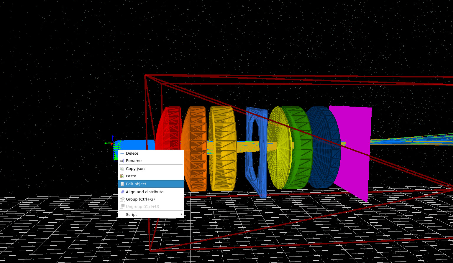
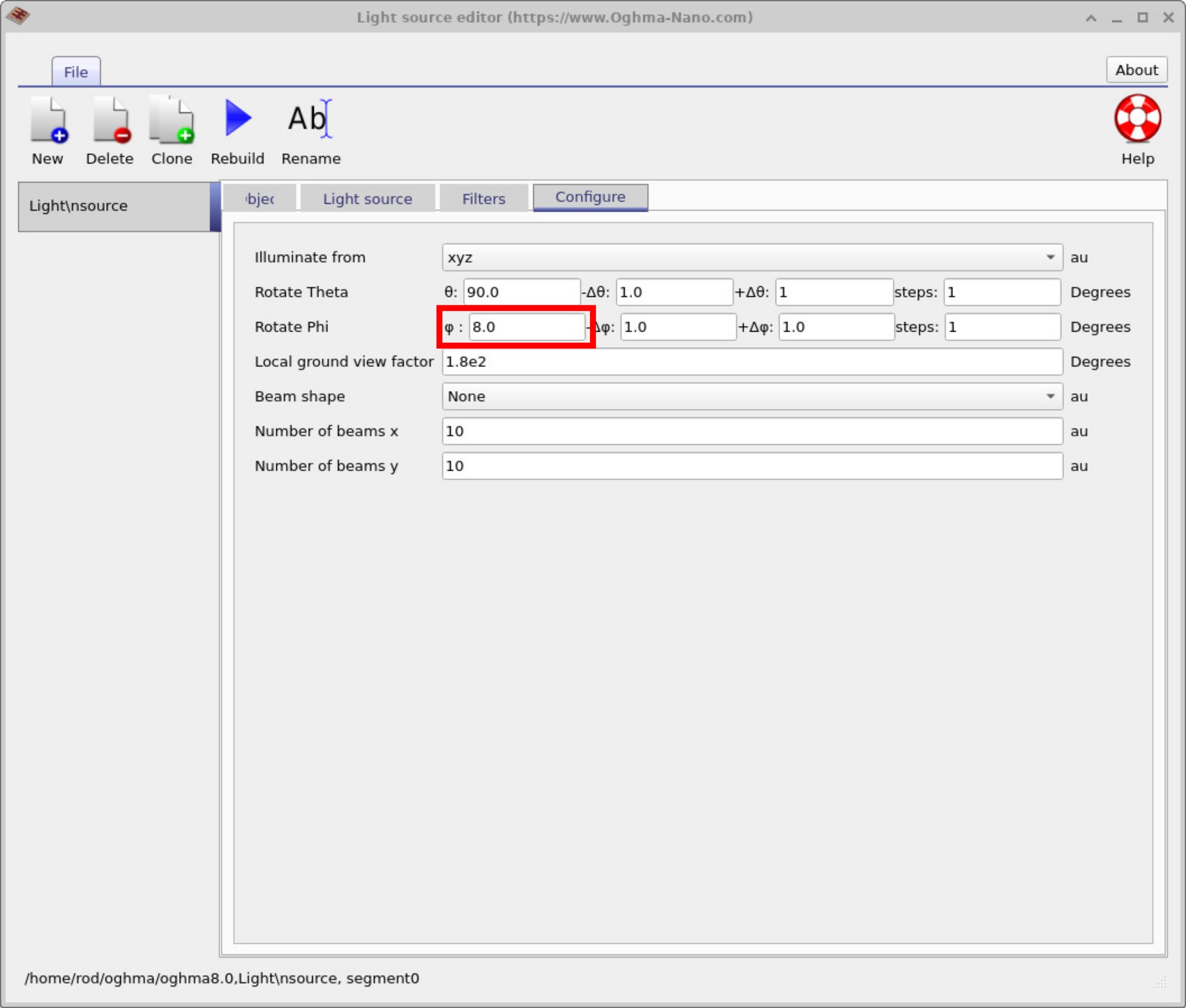
When the aperture is closed to obtain a sharper, more point-like image, a common by-product can be reduced light around the edges of the image, this is called Vignetting an example can be seen in. (??). Clipping refers to the case when rays are physically blocked by an aperture or lens edge and fail to reach the detector. Both effects are easiest to reveal when you give the rays a small field angle. In OghmaNano this is typically done using a rotation parameter such as Rotate Phi in the light source editor. To edit the light source, right-click the light source and select Edit object (??). This opens the light source editor where you can set Rotate Phi (for example to 8°) (??).
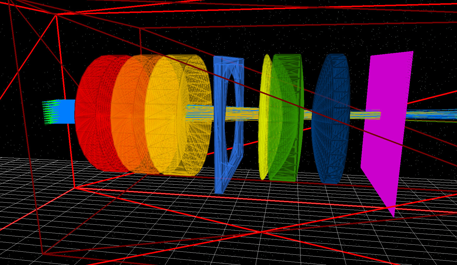
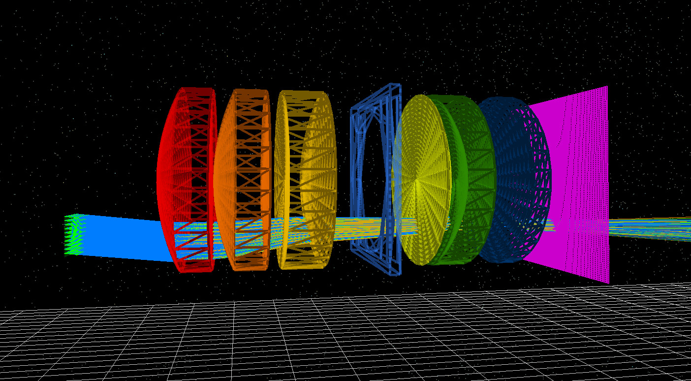
With Rotate Phi set, place the angled beam in the centre of the lens stack and run again (??). You should now see the beam propagate through the system with a controlled tilt, which makes it much easier to spot where rays are being rejected.

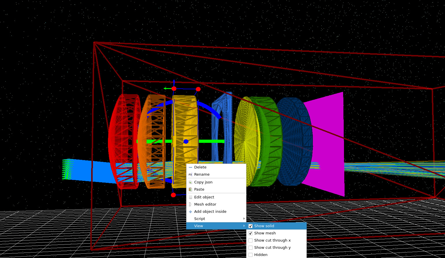
For the next run, turn off the solid rendering of the lenses so you can see ray paths inside the glass. Right-click a lens, go to View, and unselect Show solid (??). Then rerun (or just inspect the existing rays) and study how the bundle is steered surface-by-surface (??).
Now repeat the same inspection for an edge-of-pupil placement (as in Section 2), but keep the same field angle. This combination (field angle + marginal rays) is where vignetting shows up first. If rays disappear, your task is to identify where they are rejected: the stop itself, a mechanical barrel, or a clear-aperture limit of a lens element.
What you can now do (Part B)
- Locate the aperture stop (by behaviour, not by label) and explain why it globally sets the accepted ray cone for the whole system.
- Deliberately choose ray families by pupil sampling: run a clean near-axis bundle (chief/paraxial behaviour) and a matched edge-of-pupil bundle (marginal behaviour), keeping all other settings fixed.
- Diagnose “throughput vs sharpness” trade-offs without metrics by comparing 3D ray paths and detector footprints (symmetry, smear, and where energy is being lost).
- Distinguish vignetting from clipping: vignetting appears as a smooth edge falloff, while clipping produces hard cut-offs where rays are physically blocked by a stop or lens edge.
Rule of thumb — where problems show up first
- Marginal rays reveal aberrations and clipping before near-axis rays.
- Small field angles reveal vignetting before the on-axis case does.
- Hard edges in the footprint usually indicate clipping; smooth falloff usually indicates vignetting.
- If you change more than one thing at once, you lose the ability to attribute the cause.
- Do not optimise a lens until these basic checks behave in a way you can explain.
👉 Next steps: Continue to Part C, where we will compare the Cooke Triplet and the modern 200 mm prime.
For an overview of optical systems and ray-tracing simulations, see Optical systems and ray tracing overview.