Ray-tracing Tutorial (Part A): MicroLens Demo (quick start)

In this tutorial you will use OghmaNano’s ray tracer to explore a microlens array with an aperture stop and a detector. You will first run the demo in its default configuration, then enable reflections and multi-bounce ray paths so you can see stray light (unwanted rays that reach the detector by indirect paths) and ghost paths caused by multiple reflections.

1. Create a new MicroLens simulation

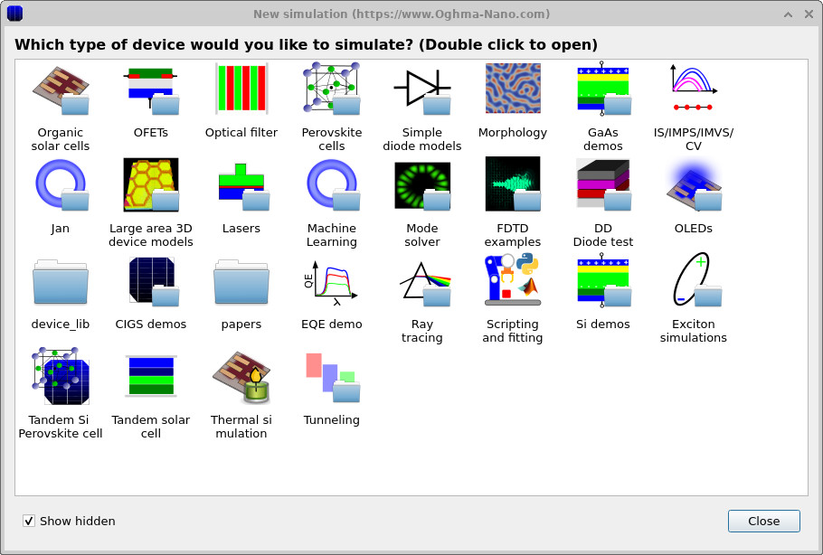
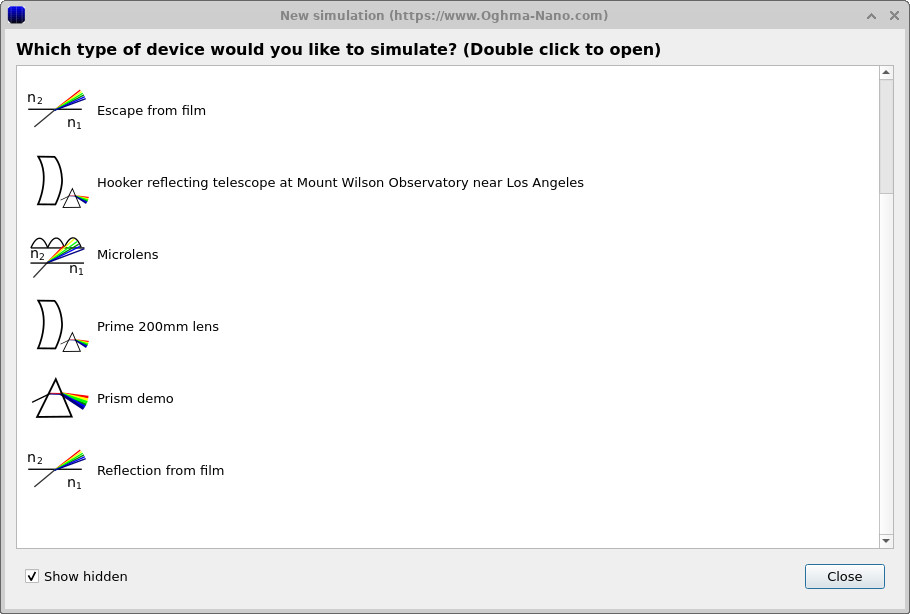
Launch OghmaNano. In the main window, click New simulation. This opens the device-type library as shown in ??. In the list of ray-tracing projects, double-click Microlens (??), then choose a directory where the simulation should be saved. As with all OghmaNano simulations, it is best to use a local folder (for example on C:\) rather than a network or cloud drive.

2. Inspect the detector, aperture and microlenses

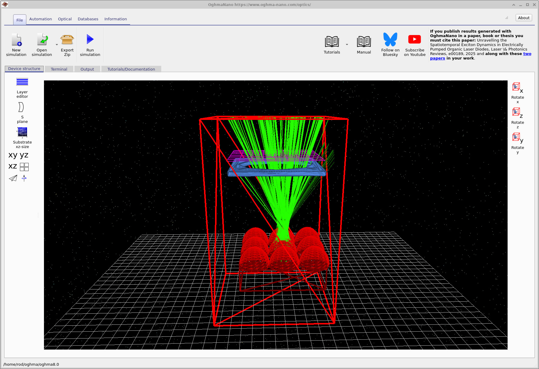
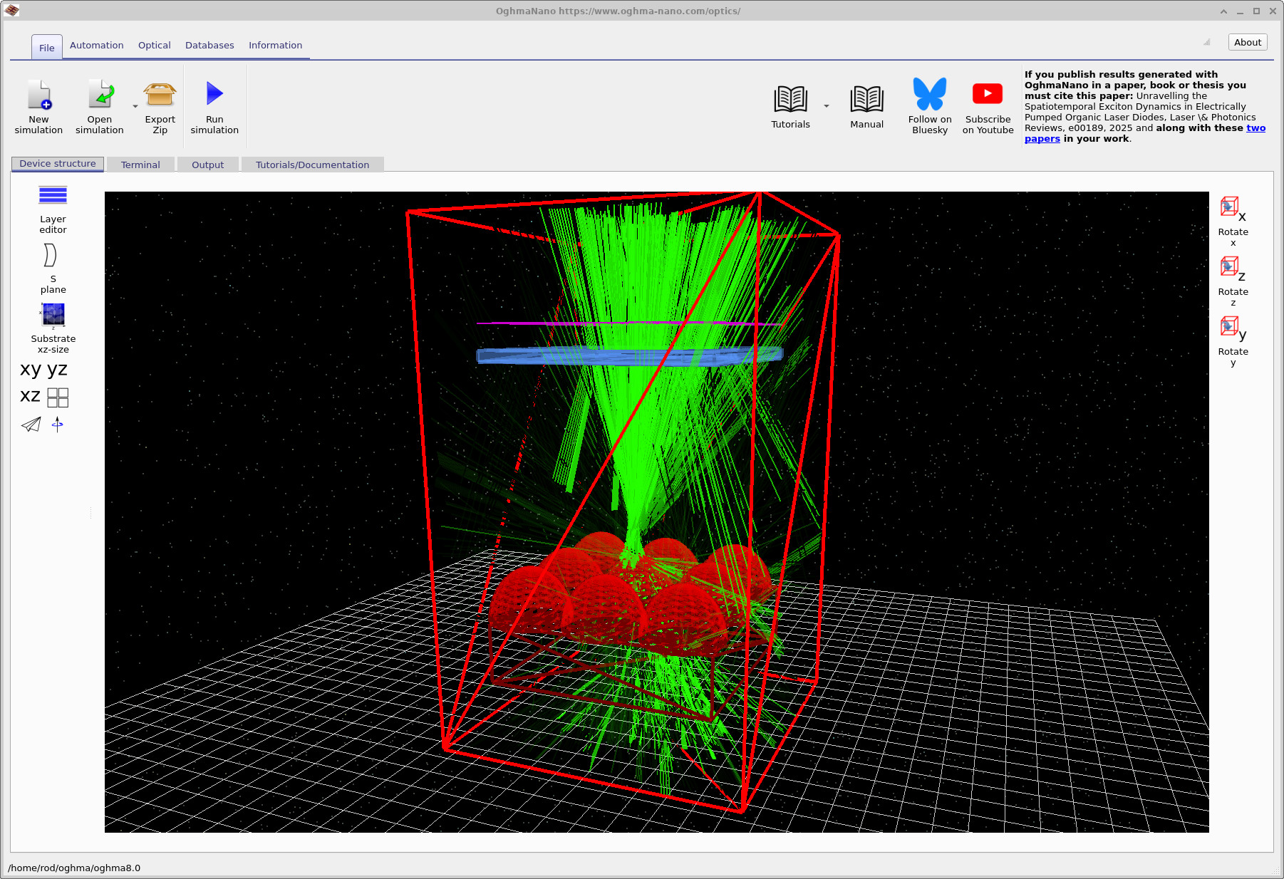
After loading the simulation, the Optical Workbench opens and displays the 3D scene (??). The scene contains: (i) a detector (purple mesh) near the top, (ii) an aperture stop (blue square plate with a circular hole), (iii) a microlens array (red domes) on a substrate. The overall scene size is approximately 4 cm × 4 cm × 5 cm: they are small lenses, but not micro-scale in the strictest sense.

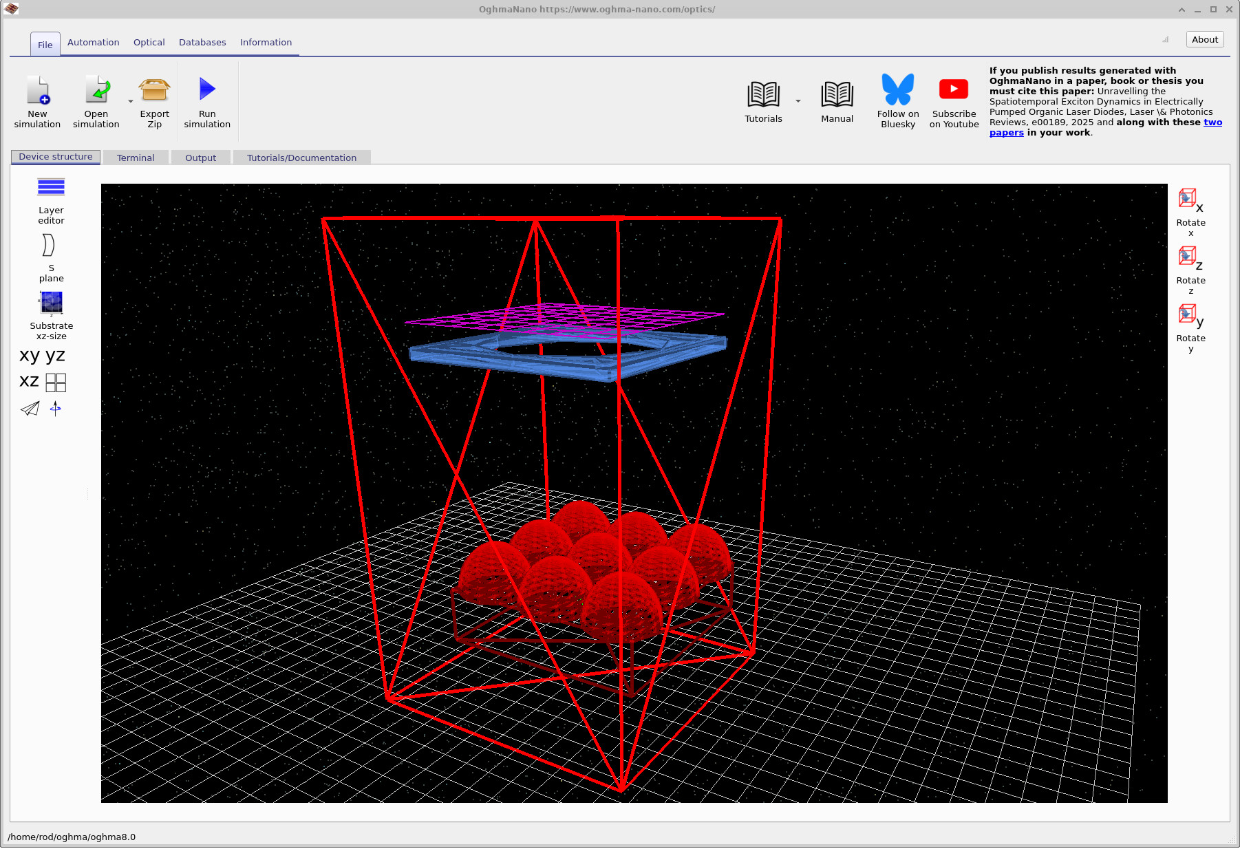
You can navigate the 3D view using the mouse:

• Left mouse button: rotate the scene.
• Right mouse button: pan the view.
• Mouse wheel: zoom in and out.

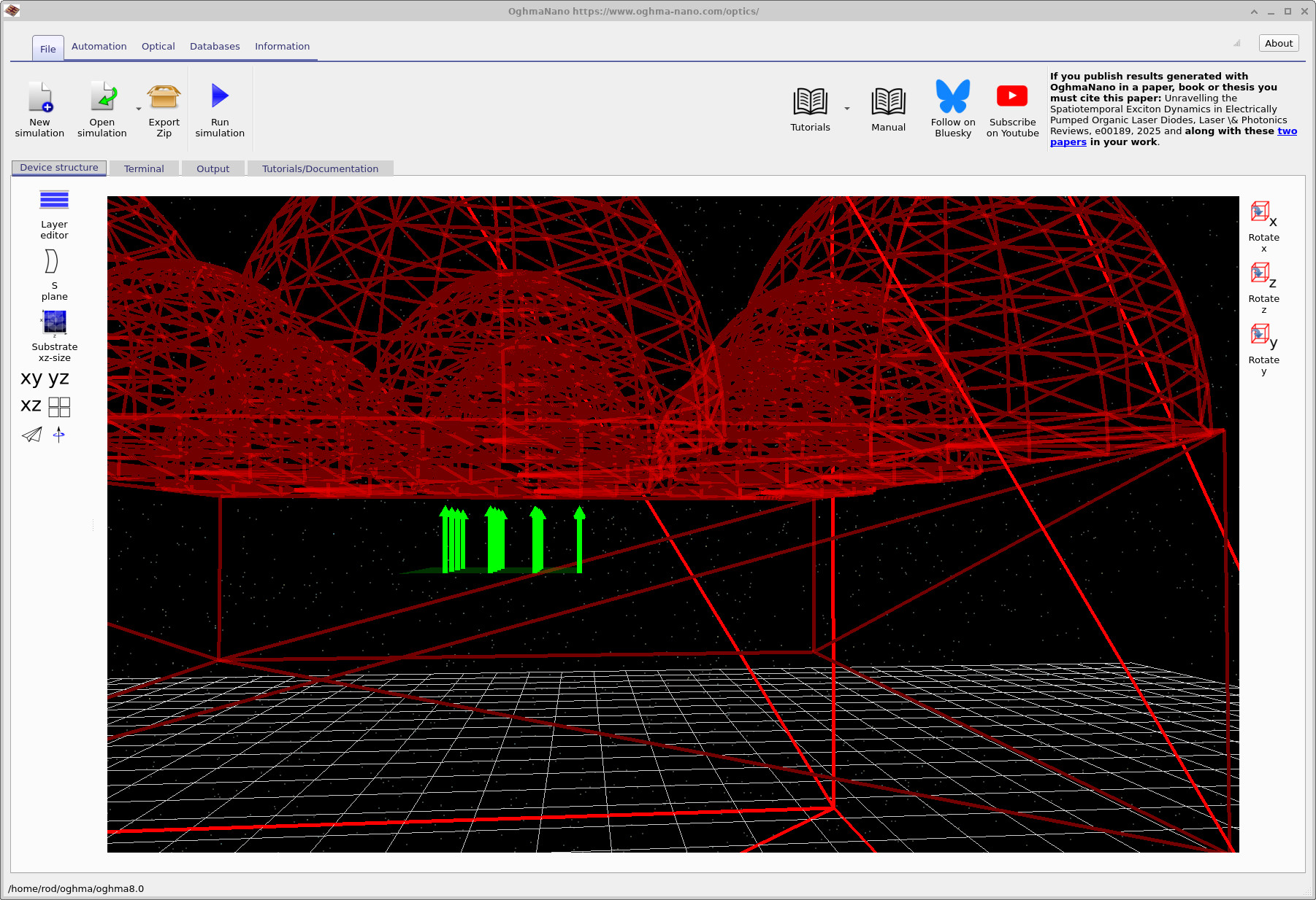
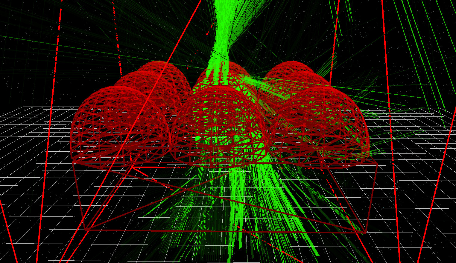
Rotate the camera so you are looking up at the underside of the microlens domes. You will see the light source region beneath the array (??). In this demo, light is emitted from below the microlenses and propagates upward toward the aperture stop and detector. You can interpret the optics above the array as a simplified “collection system” (for example, a camera or microscope objective plus stop), whose job is to accept only a subset of the rays leaving the microlens array.

3. Run the baseline ray-tracing simulation

Click Run simulation (blue play icon) or press F9. You should see rays emitted from the source, refracted by the microlens, passing through the aperture stop, and then being captured by the detector plane (??). In the default settings, the ray tracer may terminate rays early or ignore certain interactions to keep the scene clean and fast. In the next step we will deliberately increase the amount of ray physics shown so we can study indirect paths.

Step 5: Enable reflections and multi-bounce rays (stray light / ghost paths)

In practical optical systems, unwanted light can reach the detector by indirect routes: multiple reflections, grazing-incidence “skips” along surfaces, and paths that clip at the aperture stop and re-enter the system. Collectively these effects contribute to stray light, and when the same beam makes it to the detector by more than one reflection sequence it is often described as a ghost path. These effects are closely related to optical flare and veiling glare in imaging systems.

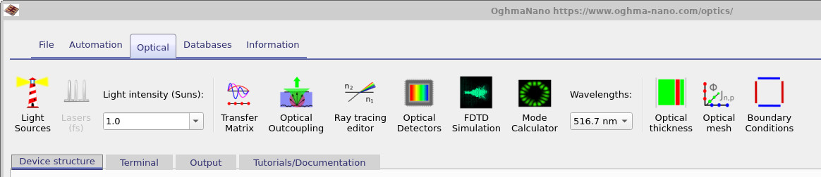
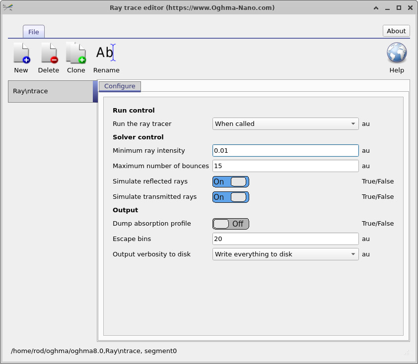
To expose these effects in the demo, open the Optical ribbon (??) and click Ray tracing editor. This opens the configuration dialog (??). Set the parameters as follows:

• Minimum ray intensity: set to 0.01. Rays are terminated once their intensity falls below 1% of the launch intensity; this prevents an explosion of very weak rays.
• Maximum number of bounces: set to 15. This allows rays to undergo multiple reflections/refractions, which is essential for visualising stray-light and ghost-path behaviour.
• Turn Simulate reflected rays On and Simulate transmitted rays On. Enabling both increases computational cost, but is necessary here because we want to see both the intended transmitted paths and unwanted reflected paths.

Now rerun the simulation (F9). With reflections and additional bounces enabled, you will see a much richer set of ray paths, including indirect rays that would normally be suppressed. The scene should resemble ?? and ??