Ray-tracing Tutorial (Part B): MicroLens Demo – Aperture filtering and source scanning
In Part A you loaded the MicroLens demo and ran a baseline ray-tracing simulation. In this part we deliberately close down the aperture stop so that only a narrow bundle of rays can reach the detector. This turns the system into a strong spatial/angle filter: most rays are rejected and only near-on-axis rays are accepted.
1. Close the aperture (reduce d0)
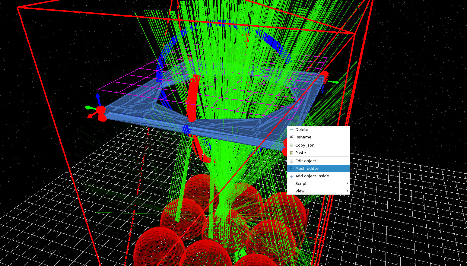
In the 3D view, right-click on the aperture stop (the blue plate with a hole) and open the Mesh editor
as shown in ??.
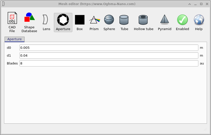
This opens the aperture editor window
(??),
where you can control the hole size. Set D0 to 0.005 m.
This effectively closes the aperture, strongly limiting which rays can pass through to the detector.
In this respect the aperture plays a role similar to the pinhole in a confocal microscope or to
field stops used in other optical instruments: only rays arriving from a narrow range of positions and angles
are accepted, while off-axis and stray light is rejected.
0.005 m to close the hole.
Rerun the simulation (F9). You should now see that most rays are rejected: only a small fraction of light makes it through the aperture and reaches the detector plane (purple grid), as shown in ??. Conceptually, the aperture is selecting rays based on where they come from and what angle they travel at: rays arriving too far off-axis (or originating from the “wrong” region of the microlens array) are blocked.
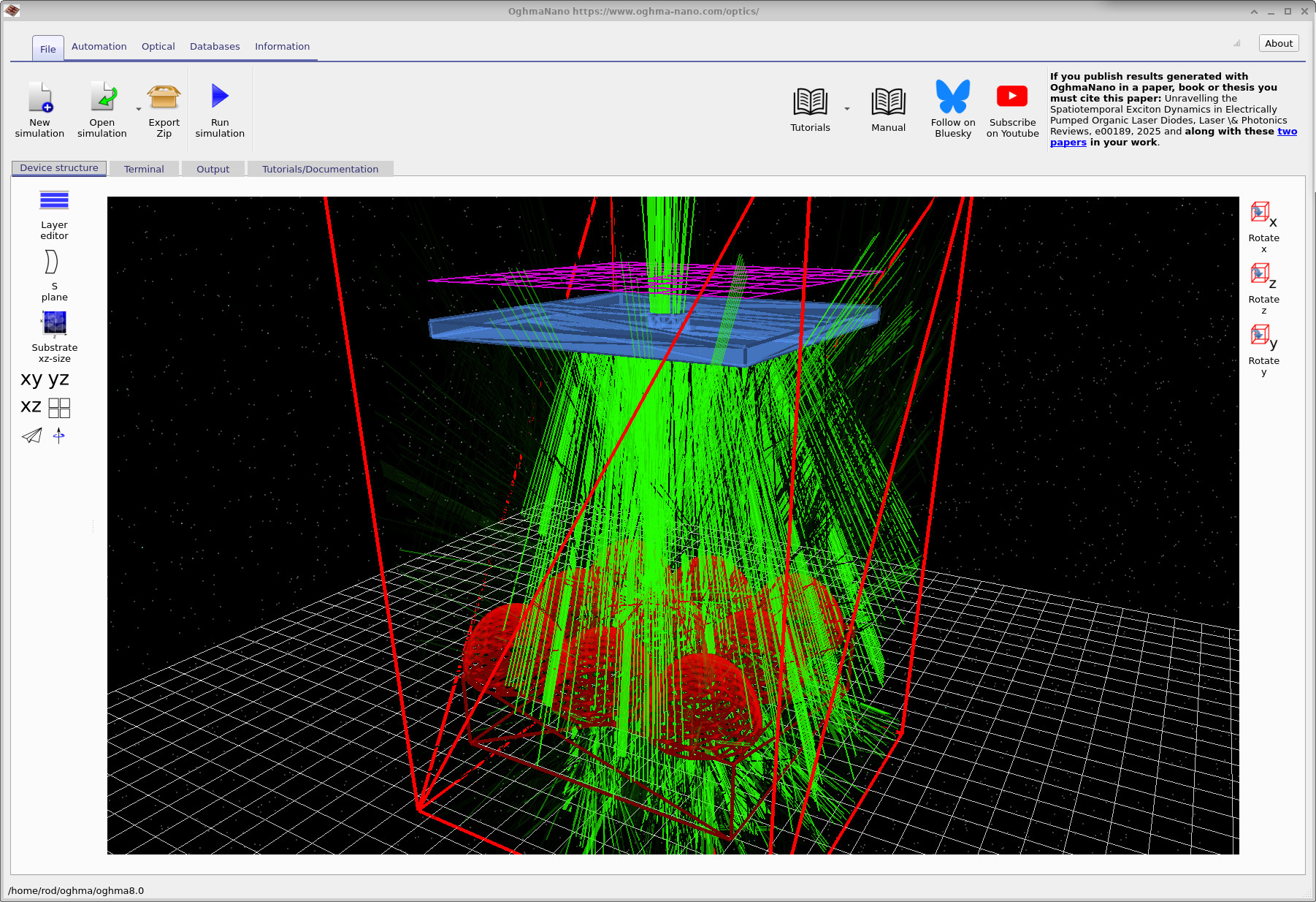
d0 = 0.005 m), most rays are blocked and only a narrow bundle reaches the detector.
2. Scan the source position and observe acceptance
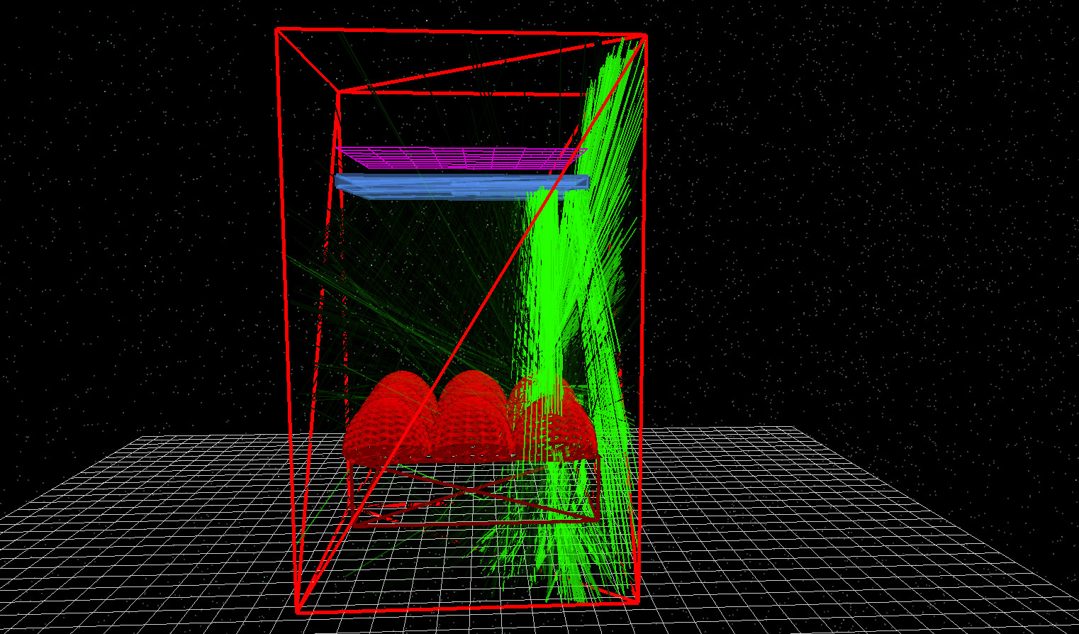
Reorient the camera so you can clearly see the source region and the microlenses, similar to ??. Using the mouse, move the optical source laterally across the simulation window and try to find the point at which rays no longer reach the detector. With the aperture nearly closed, there will be a range of source positions for which rays can still pass through the hole and reach the detector, and beyond some offset the detector will receive essentially no light.
To quantify how much light reaches the detector, switch to the Output tab, open detector0, and then open
detector_efficiency0.csv. This file plots wavelength against the fraction of emitted light accepted by the detector.
Detectors and their outputs are covered in other tutorials in more detail; here we use the efficiency spectrum as a compact measure of
optical acceptance.
Confocal-style optical filtering (pinhole analogy)
-90 to +90 with 20 steps).
A confocal microscope improves image contrast by using a pinhole placed so that light from the focal region is preferentially transmitted, while out-of-focus and off-axis light is rejected. This is usually introduced in terms of depth (axial) sectioning, but the same principle also applies laterally: an aperture can act as a spatial filter that only admits light from a limited region and angular range.
In this MicroLens demo the aperture stop plays a similar role to the confocal pinhole: it enforces a strict acceptance condition. When you scan the source sideways, you are effectively measuring a lateral acceptance function of the optical system. Closing the aperture suppresses background and stray rays, but it also makes the detector signal highly sensitive to source position and emission angle.
3. Emit light over a wider angular range
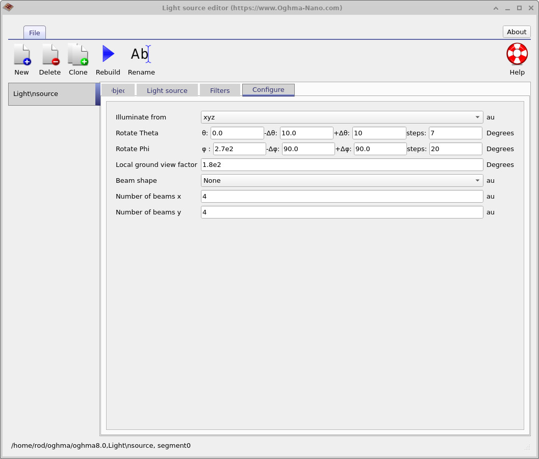
Next we will make the source emit into a broader set of directions. Right-click on the light source to open the source editor
(??).
Increase the Phi angular span so that light is emitted from -90 to +90 degrees using 20 steps.
This will emit rays in many more directions.
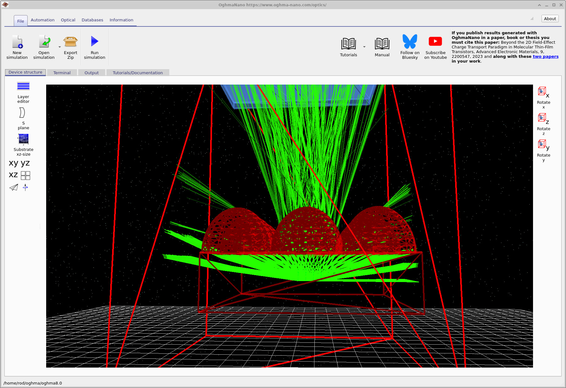
Rerun the simulation. You should see many more rays, including rays that escape sideways as well as upward through the aperture,
as shown in ??.
If you inspect detector0/detector_efficiency0.csv again, the detector acceptance will typically be very low:
most of the emitted light does not meet the geometric constraints needed to pass through the stop and reach the detector.
Why efficient light collection is hard
This behaviour reflects a general difficulty in optical systems: once you introduce apertures, baffles, finite detector sizes, or limited numerical aperture, you enforce a strict acceptance condition in position and angle. Light emitted over a broad angular distribution (for example from scattering, diffuse emitters, fluorescence, or rough surfaces) is intrinsically hard to collect efficiently without either (i) a high-NA collection optic, (ii) an etendue-matched detector, or (iii) accepting more background and stray light.
Practical examples include imaging systems fighting flare and veiling glare (where stray light washes out contrast), microscope systems trading signal for optical sectioning (the confocal pinhole rejects background but also rejects signal), and sensors behind windows or housings where internal reflections create ghost paths. The MicroLens demo makes these trade-offs visible: close the aperture and you suppress background, but you also make the system far less forgiving to source position and emission angle.
👉 Next steps: Continue to Part C where we will modify the geometry (for example changing dome profiles and adding surface micro-structure) and observe how those changes alter acceptance and stray-light behaviour.
For an overview of optical systems and ray-tracing simulations, see Optical systems and ray tracing overview.