Ray-tracing Tutorial (Part C): MicroLens Demo – Shape engineering (Gaussian and spheres)

In Part B we used the aperture stop as a strong spatial/angle filter and saw how sensitive detector acceptance can be. In this final part we change the geometry of the microlens features themselves. The goal is not to “optimise” a lens, but to build intuition: surface shape controls the angular distribution of escaping rays, and that directly determines how much light the detector can accept through a finite aperture.

1. Changing the shape of the lenses

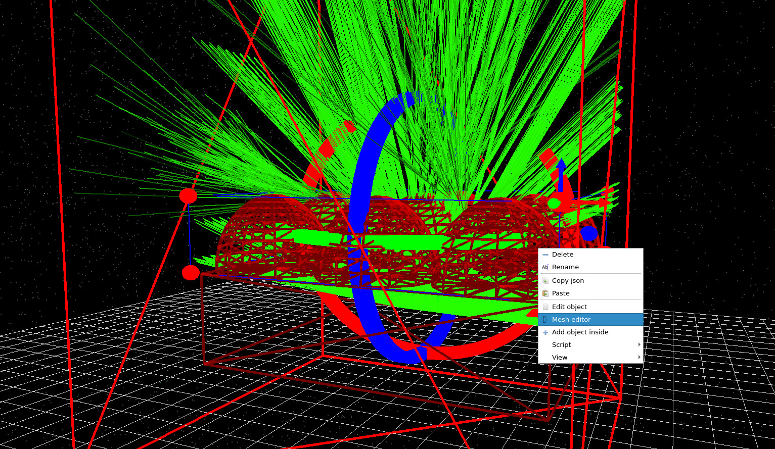
Right-click on the microlens object in the 3D scene and select Mesh editor (??). This opens the microlens mesh editor window (??), where you can change the geometry by selecting a different shape from the database.

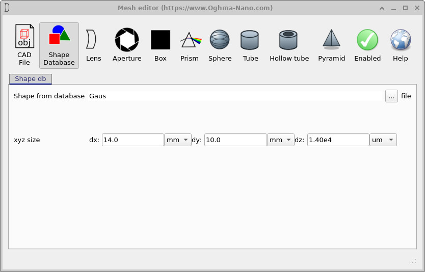
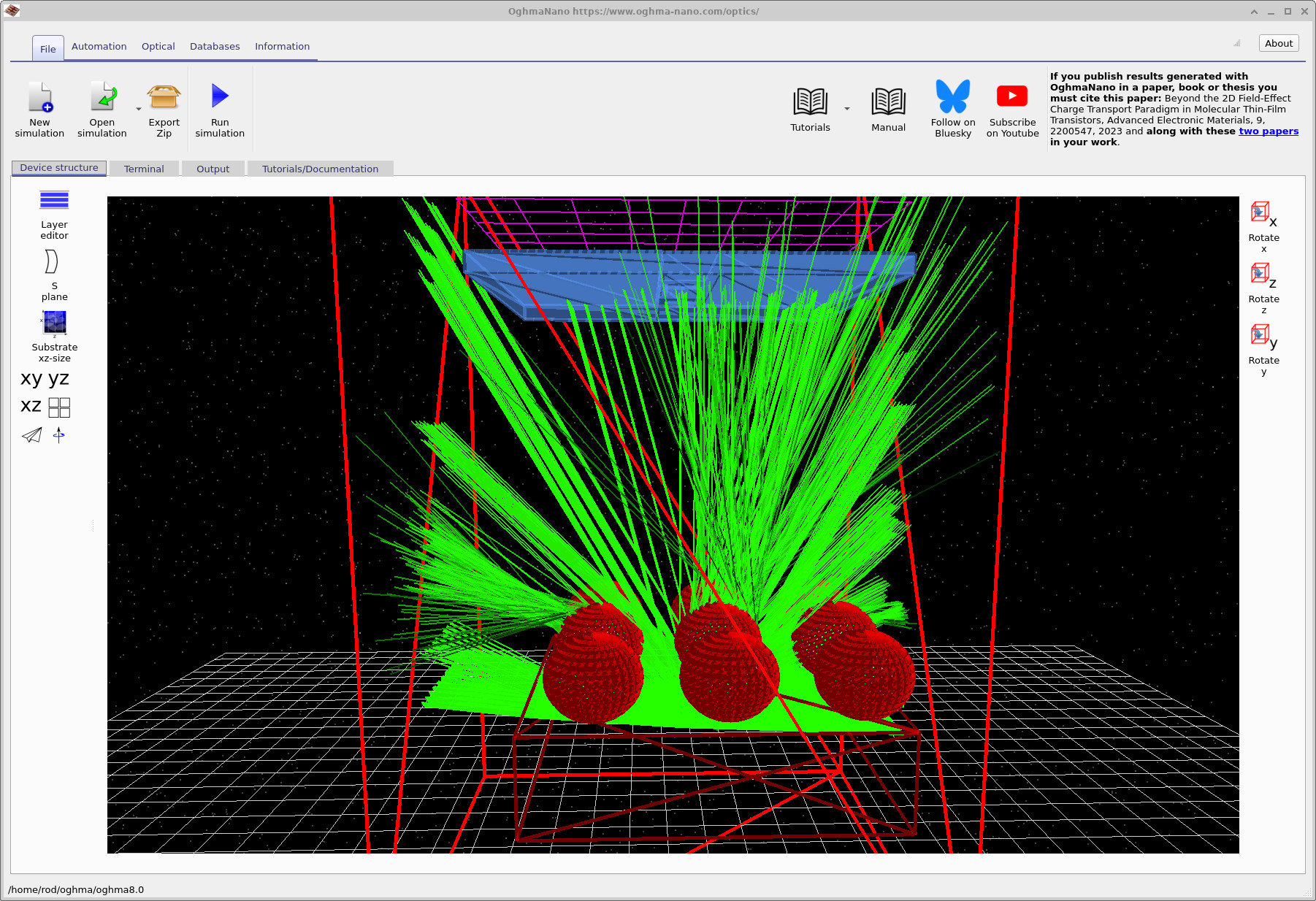
In the mesh editor, change Shape from database from the default dome to gauss, then rerun the simulation. Your result should look similar to ??. Notice how the ray bundle changes: the Gaussian profile tends to redistribute rays differently, and in this particular setup you will often find that less light makes it through the detector hole. That is a geometric effect: the detector can only accept rays within a limited position/angle window, so any change that increases divergence (or shifts rays laterally) reduces acceptance.

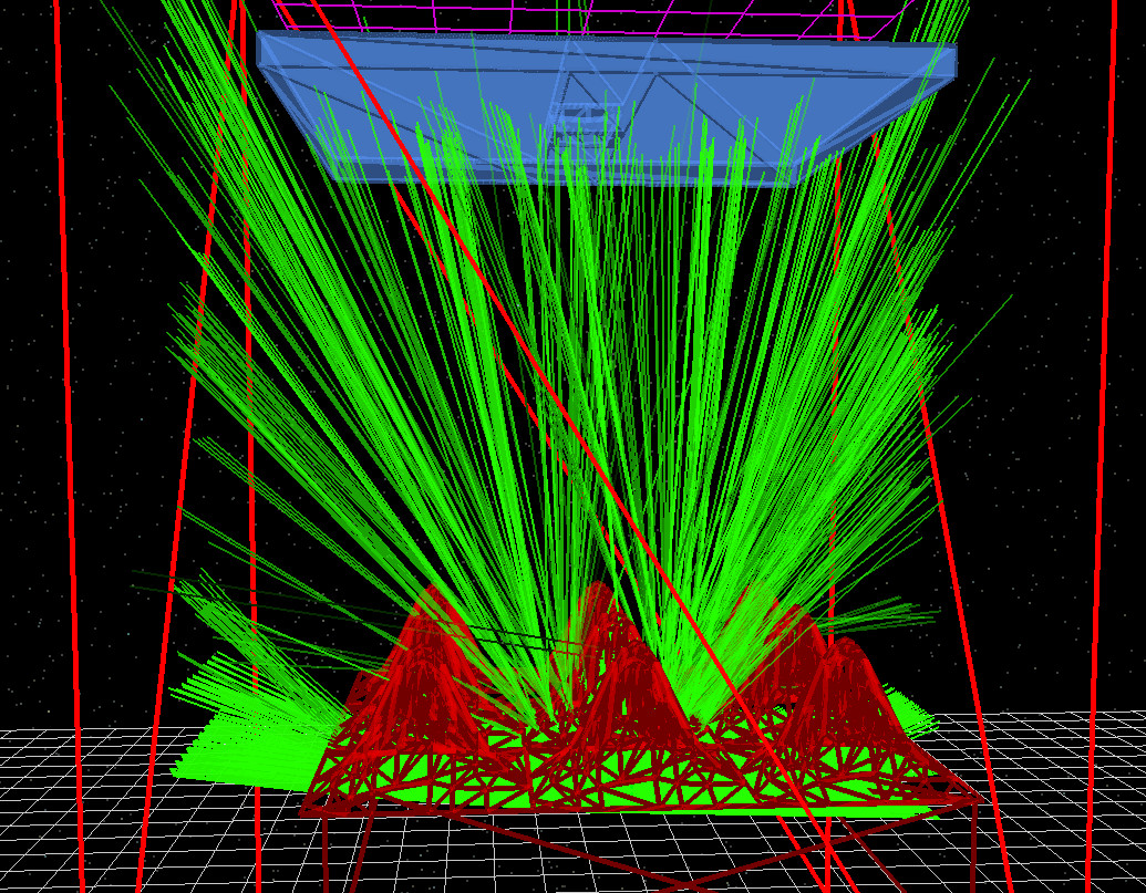
Next, experiment with a more extreme geometry. In the mesh editor, switch the microlens object to balls by selecting the sphere icon and rebuilding/rerunning the simulation. The result can be seen in ??. Compared to a smooth lens surface, spherical features behave more like strong curvature elements that inject a wider range of ray angles, which can dramatically increase sideways leakage and stray paths.

What to take away from Gaussian and spheres

The key lesson is that “extraction efficiency” is not just about how much light leaves a surface, but about where it goes. In these scenes the detector is not an infinite hemisphere: it sits behind a finite aperture stop, so only a subset of ray angles are useful. A surface that produces a tight, on-axis bundle can look “bright” at the detector even if total escaping power is similar, because it matches the system’s acceptance.

The Gaussian shape tends to soften the surface curvature distribution compared to a simple dome, which can change the local refraction angles across the feature. Depending on your geometry, that can increase divergence, move the caustic, or shift where rays cross the aperture plane. The net effect is often a drop in accepted power: more rays exist, but fewer fall into the small phase-space window that the detector can collect. In other words, you have changed the etendue matching between source, microlens and detector.

The spheres (balls) case is deliberately “non-optical” in the classical sense: it introduces strong curvature and multiple opportunities for rays to be launched at large angles. This tends to create more stray light paths and lateral leakage, which is exactly the kind of behaviour that real optical designers try to suppress with smooth surfaces, careful stop placement, and baffles. It is a useful stress test: if your detector signal collapses when you introduce spherical features, that is telling you the system is acceptance-limited and highly sensitive to angular scatter.

Practically, this is also why microlens arrays in imaging systems are engineered for the specific sensor stack and stop geometry: you are not designing “a lens”, you are designing an angular transformer that maps a source distribution into the acceptance of the downstream optics. The point of this demo is that OghmaNano lets you explore that mapping visually before you commit to any metrics or optimisation workflow.