IMPS Simulation Tutorial

1. Introduction

IMPS (Intensity-Modulated Photocurrent Spectroscopy) probes how the photocurrent of a device responds to a small sinusoidal modulation of the incident light. In practice, the illumination is written as \( I_{\mathrm{light}}(t) = I_{0} + \Delta I \, e^{i\omega t} \), and the resulting photocurrent response can be expressed as \( J(t) = J_{0} + \Delta J \, e^{i(\omega t + \phi)} \).

The ratio \[ H(\omega) = \frac{\Delta J(\omega)}{\Delta I(\omega)} \] defines the complex IMPS transfer function, whose magnitude and phase provide insight into the underlying physics. At high frequencies, limited carrier collection suppresses the response, while at low frequencies the photocurrent follows the light modulation more closely. Features such as arcs and peaks in Nyquist or Bode plots can be traced back to charge transport times, recombination lifetimes, and interfacial kinetics.

With OghmaNano, you can simulate IMPS directly on a device model and generate Nyquist and Bode plots that mirror experimental data. This allows you to disentangle the roles of transport, recombination, and contact resistances, and to test hypotheses before or alongside laboratory measurements.

2. Getting started

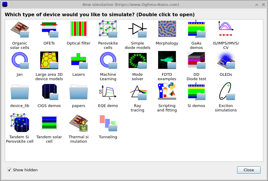
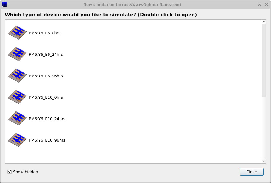
To begin, open the New simulation window (see ??) and double-click the Organic solar cells category. This folder contains a range of OPV demo devices suitable for running IMPS simulations. From the list that appears (see ??), select a PM6:Y6 demo device (for example, PM6:Y6_E6_0hrs). This provides a preconfigured project with sensible defaults, so you can run IMPS directly without building a device from scratch.

3. Examine the IMPS setup

From the Editors ribbon in the main window, open the FX Domain Editor, then click the IMPS tab (Intensity-Modulated Photocurrent Spectroscopy).

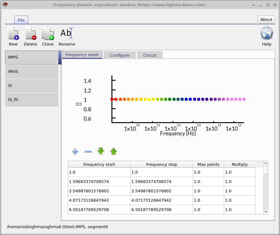
Check the Frequency mesh to see which frequency points will be simulated (??). Here the mesh is specified as individual points (useful for matching experimental frequencies), but you can also use a continuous range with a start/stop frequency and a maximum number of points. To increase spacing between points, adjust the Multiply factor from 1.0 to a value > 1 (e.g., 1.05) for geometric spacing; values < 1 compress spacing.

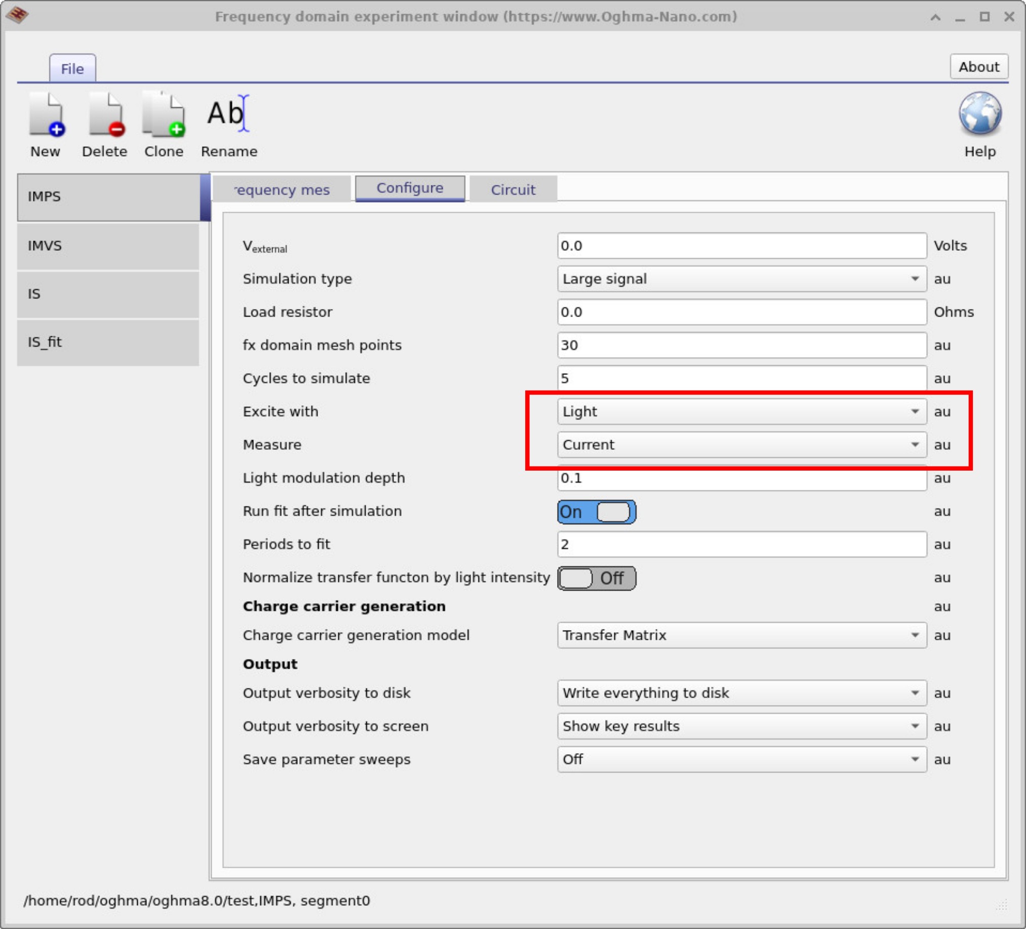
Next, open the Configure tab (??). For IMPS, set Excite with to Light and Measure to Current. Keep the external bias Vexternal at 0 V for short-circuit IMPS, and choose a small Light modulation depth (e.g., 0.1 in relative units) to remain in the linear response regime. These parameters define a standard IMPS experiment in OghmaNano.

4. Setting the simulation mode

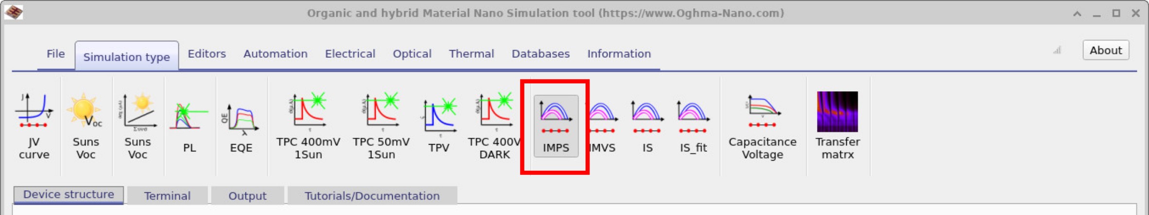
All frequency-domain simulations that are defined in the FX Domain Editor (e.g. IMPS, IMVS, and IS) will appear as buttons on the Simulation type ribbon. Before you run the IMPS simulation, make sure the IMPS mode button is selected (depressed); otherwise a different mode may run (see ??).

4. Running the simulation and viewing outputs

From the main simulation window, open the File ribbon and click Run simulation (??). You can also press F9 as a shortcut while the main window is active.

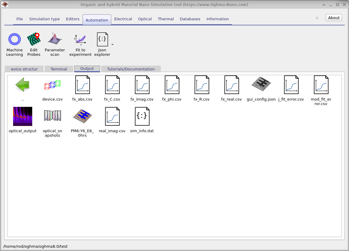
When the IMPS run finishes, go to the Output tab to find the generated result files (??). Typical files include fx_real.csv, fx_imag.csv, fx_phi.csv, and real_imag.csv for plotting Bode and Nyquist responses.

5. Reading Bode & Nyquist plots

Once the IMPS simulation has finished, you can explore the results by double-clicking the output files in the Output tab. Before you begin, remember that you can press L while viewing a plot to toggle a logarithmic y-axis, and Shift+L to toggle a logarithmic x-axis. These shortcuts make it easier to highlight features across many orders of magnitude, and they are particularly useful for IMPS data where both fast and slow processes are present.

• fx_real.csv – Bode (real) plot (??): shows the in-phase component of the photocurrent. In this device the real part steadily decreases with frequency, confirming that carriers are collected efficiently at low frequency but cannot keep up once modulation exceeds around \(10^5\)–\(10^6\) Hz. This roll-off marks the onset of transport/recombination limitations.
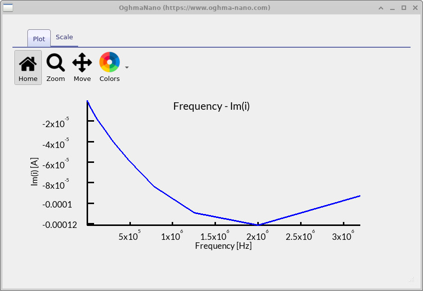
• fx_imag.csv – Bode (imag) plot (??): shows the out-of-phase component. The negative dip seen here around \(1.5 \times 10^6\)–\(2.0 \times 10^6\) Hz pinpoints the dominant recombination or transport timescale. The frequency of this dip corresponds to a time constant of \(\tau \approx 1 / (2 \pi f) \sim 0.1\ \mu\text{s}\), meaning carriers respond on sub-microsecond timescales.
• fx_phi.csv – Bode (phase) plot (??): shows how far the photocurrent lags behind the modulated light input. At low frequency the phase is near 0°, confirming near-instantaneous response. Around the MHz range it shifts strongly negative (down to ~−80°), indicating that recombination dominates and the device response is increasingly delayed.
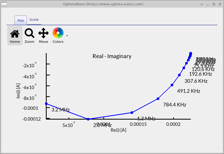
• real_imag.csv – Nyquist plot (??): presents the same information in the complex plane. The single arc centred near 200 kHz–1 MHz shows that one RC-like process dominates the device response. Its relatively small size suggests recombination is significant but not catastrophic, and the frequency labels align with the same timescale observed in the Bode plots.

Taken together, the IMPS plots show that this device responds efficiently to slow light modulation, with carriers being well collected at low frequencies. The clear features around 1–2 MHz mark the dominant recombination/transport process, with a characteristic time constant of order \(\tau \sim 0.1\ \mu\text{s}\). At higher frequencies the photocurrent rolls off steeply, as the device cannot respond any faster. Overall, the spectrum reveals a single, well-defined dynamic bottleneck: the device behaves like a simple RC system where transport and recombination set an effective speed limit for converting modulated light into photocurrent.

Below you’ll find an overview of the key IMPS output files and what each one contains.

6. Summary & next steps

In this tutorial you learned how to set up and run an IMPS (Intensity-Modulated Photocurrent Spectroscopy) simulation in OghmaNano, and how to interpret the resulting Bode and Nyquist plots. You saw how low-frequency behaviour reflects efficient carrier collection, how mid-frequency features highlight recombination or transport bottlenecks, and how high-frequency roll-off signals the device’s dynamic limits. The same workflow can be applied not only to organic solar cells but also to perovskites, tandems, and other optoelectronic devices where photocurrent dynamics are important. For more advanced analysis, export the CSV data to extract carrier lifetimes, fit kinetic models, or benchmark against experimental measurements.