IMVS Simulation Tutorial

1. Introduction

IMVS (Intensity-Modulated Photovoltage Spectroscopy) examines how the open-circuit voltage of a device responds to a small sinusoidal modulation of the incident light. In this case, the illumination can be written as \( I_{\mathrm{light}}(t) = I_{0} + \Delta I \, e^{i\omega t} \), and the device responds with a time-dependent voltage \( V(t) = V_{\mathrm{oc},0} + \Delta V \, e^{i(\omega t + \phi)} \).

The ratio \[ H(\omega) = \frac{\Delta V(\omega)}{\Delta I(\omega)} \] defines the complex IMVS transfer function, which captures how efficiently the device converts a modulated optical input into a photovoltage response. At low frequencies, the voltage follows the light modulation closely, while at higher frequencies the response rolls off due to finite carrier lifetimes and recombination pathways. The frequency at which the imaginary part peaks is directly related to the effective carrier lifetime, \(\tau \approx 1/(2\pi f_{\mathrm{peak}})\).

Using OghmaNano, you can simulate IMVS directly on a device model and generate Bode and Nyquist plots comparable to experimental measurements. This enables you to identify recombination-limited processes, assess the impact of contacts and transport layers, and link the observed lifetimes to microscopic physics. As with IS and IMPS, these simulations allow you to test hypotheses virtually before committing to laboratory experiments.

2. Getting started

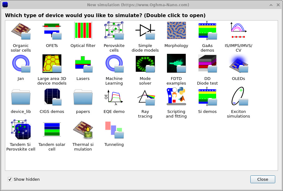
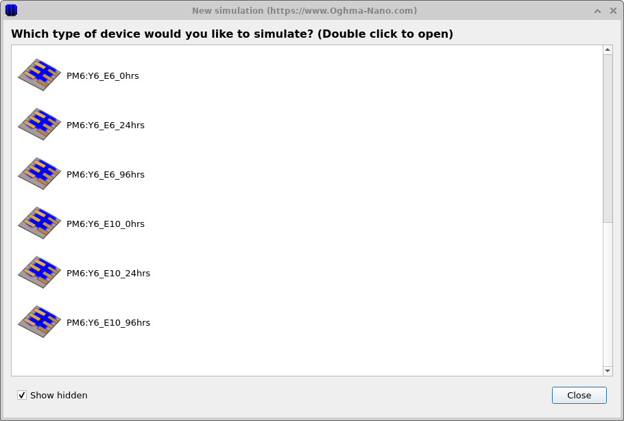
Begin by opening the New simulation window (see ??) and select the Organic solar cells category. This contains a set of demonstration OPV devices that can be used as ready-made starting points for IMVS studies. From the list of available templates (see ??), choose a PM6:Y6 example device (for instance, PM6:Y6_E6_0hrs). This template comes preconfigured with sensible defaults, allowing you to run IMVS immediately without having to build a full device structure from scratch.

OghmaNano 'New simulation' window with categories; Organic solar cells highlighted. — *New simulation* window — open the **Organic solar cells** category.

Template list showing PM6:Y6 demo devices; one entry provides a preconfigured IMVS setup. — Template list: choose a **PM6:Y6** device to run an IMVS simulation.

3. Examine the IMVS setup

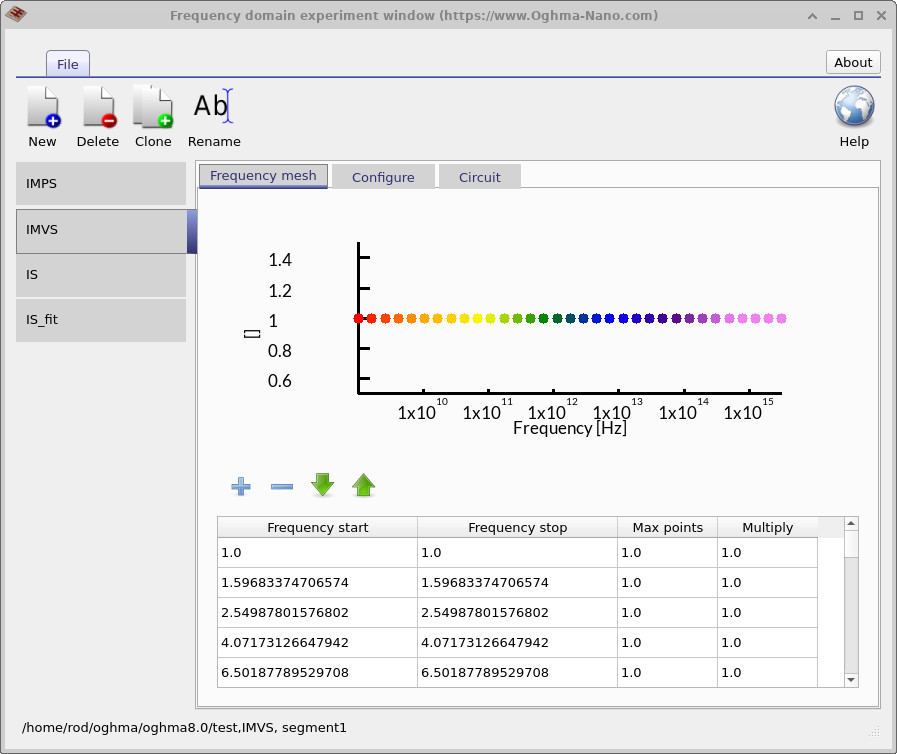
From the Editors ribbon in the main window, open the FX Domain Editor, then click the IMVS tab (Intensity-Modulated Photovoltage Spectroscopy).

Check the Frequency mesh to see which frequency points will be simulated (??). In this example, the mesh is listed as individual points (helpful if you want to match specific experimental frequencies), but you can also define a continuous range by setting a start/stop frequency and the maximum number of points. To change the spacing between points, adjust the Multiply factor: values greater than 1 (e.g., 1.05) give geometric spacing, while values below 1 compress the spacing.

FX domain editor on the IMVS tab showing the Frequency mesh table with listed frequency points. — **Frequency mesh** tab: define frequency points or ranges for IMVS simulations.

Configure tab for IMVS: simulation type, mesh points, 'Excite with: Light', 'Measure: Voltage', and light modulation depth. — **Configure** tab: set *Excite with* = Light, *Measure* = Voltage, choose modulation depth, and other options.

Circuit tab showing an equivalent circuit set to open circuit for IMVS simulation. — **Circuit** tab: defines the operating condition. For IMVS, the circuit is set to *open circuit*, since the technique measures photovoltage dynamics without external load.

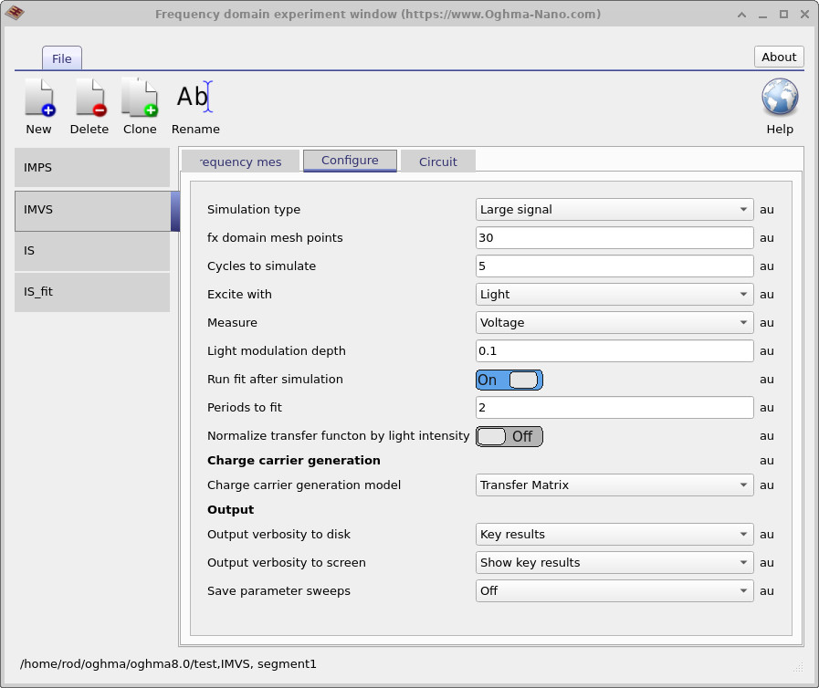
These settings together define an IMVS (Intensity-Modulated Photovoltage Spectroscopy) run. In the Frequency Domain Editor you’ll see the simulation type labelled as IMVS, although you can name the project itself however you wish. What makes this setup IMVS is the specific combination of conditions: excitation is applied with Light, the response is measured as Voltage, the Light modulation depth is set to 0.1 V, and in the Circuit tab the load is fixed to open circuit. Together these settings replicate the way IMVS is performed experimentally — applying a small sinusoidal modulation of light and tracking the resulting photovoltage under open-circuit conditions.

4. Setting the simulation mode

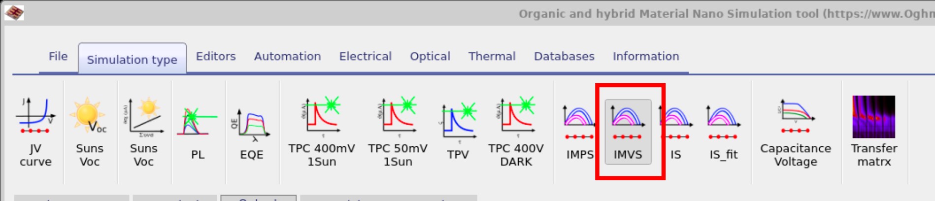
All frequency-domain simulations defined in the FX Domain Editor (such as IMPS, IMVS, and IS) appear as selectable buttons in the Simulation type ribbon. Before running an IMVS simulation, check that the IMVS button is selected (depressed); otherwise, the software may attempt to run a different mode instead (see ??).

Simulation type ribbon in OghmaNano showing IMPS, IMVS, IS, and related buttons; IMVS is highlighted to indicate it should be selected. — Simulation type ribbon: ensure **IMVS** is selected before starting the simulation.

4. Running the simulation and viewing outputs

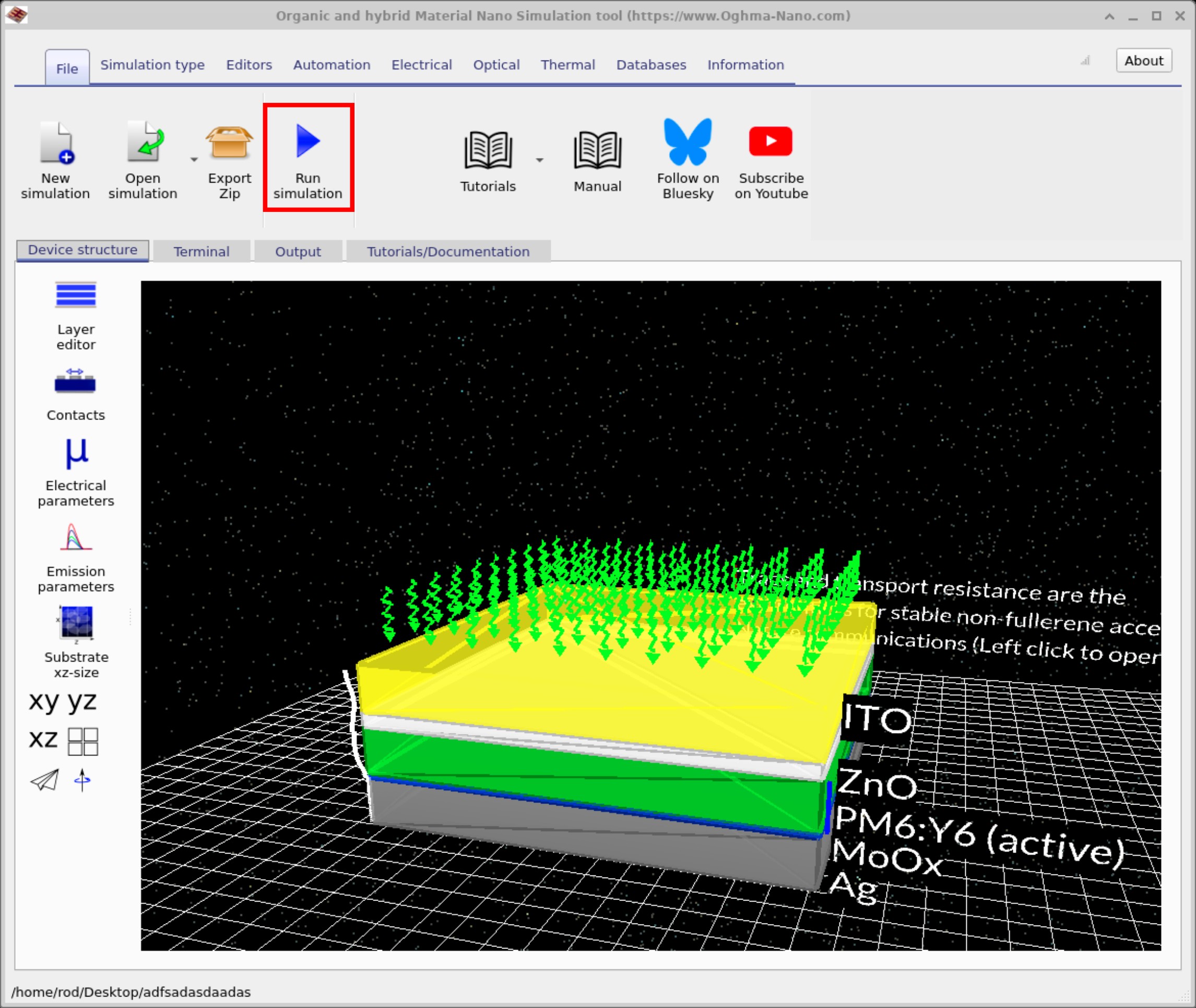
From the main simulation window, open the File ribbon and click Run simulation (??). As a shortcut, you can also press F9 while the main window is active.

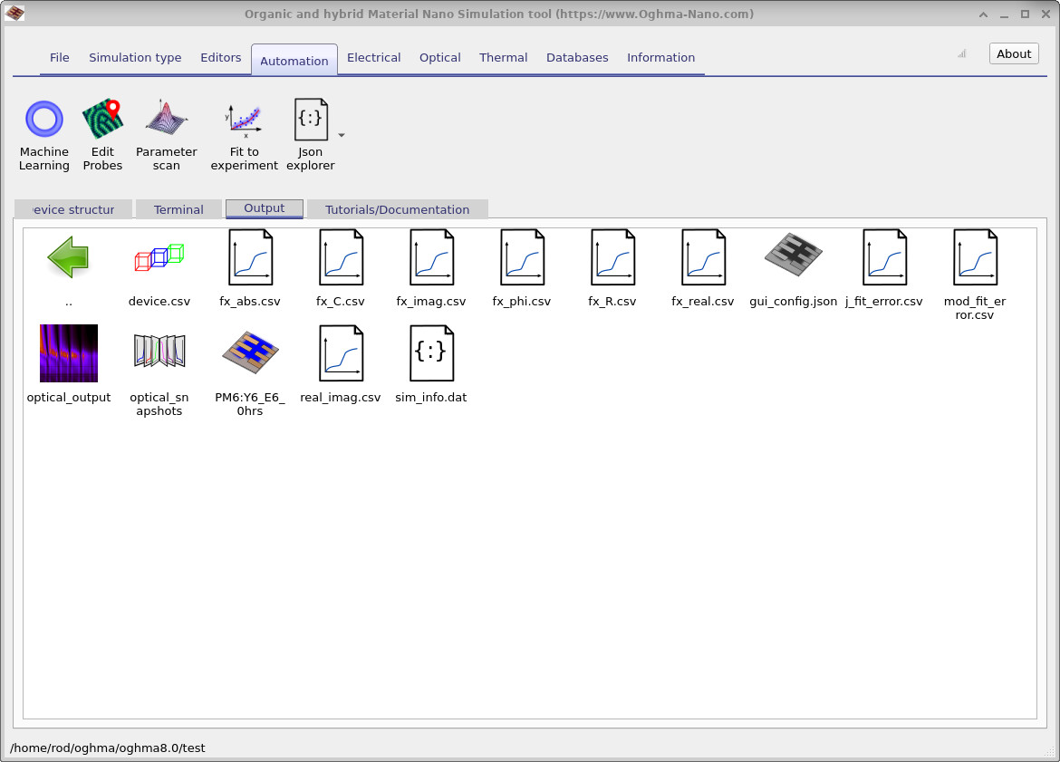
Once the IMVS run has finished, switch to the Output tab to view the generated results (??). The key files include fx_real.csv, fx_imag.csv, fx_phi.csv, and real_imag.csv, which you can use to plot Bode and Nyquist diagrams of the voltage response. Additional CSV files (e.g., fx_abs.csv, fx_C.csv, fx_R.csv) provide further analysis options.

Main OghmaNano window showing the device structure with the Run simulation button highlighted. — Main window: click **Run simulation** to start the IMVS calculation.

Output tab in OghmaNano showing IMVS result files such as fx_real.csv, fx_imag.csv, fx_phi.csv, and real_imag.csv. — Output tab: IMVS result files (e.g., `fx_real.csv`, `fx_imag.csv`, `fx_phi.csv`, `real_imag.csv`) are saved here for analysis.

5. Reading Bode & Nyquist plots

IMVS Bode plot: real (in-phase) photovoltage response versus frequency; low-f plateau with high-f roll-off. — Bode (real): in-phase photovoltage, \(\mathrm{Re}[V]\) vs. frequency (`fx_real.csv`).

IMVS Bode plot: imaginary (out-of-phase) photovoltage showing a clear peak around 0.1–0.3 MHz. — Bode (imag): out-of-phase photovoltage, \(\mathrm{Im}[V]\) vs. frequency (`fx_imag.csv`).

IMVS Bode plot: phase of the photovoltage response increasing toward ~80° across the MHz range. — Bode (phase): phase of \(V\) vs. frequency (`fx_phi.csv`).

IMVS Nyquist plot (−Im(V) vs Re(V)) showing a single semicircle with apex near 120–200 kHz. — Nyquist: −Im(V) vs. Re(V) with frequency markers (`real_imag.csv`).

After the IMVS run completes, double-click the output files in the Output tab to open the plots. While viewing any plot, press L to toggle a logarithmic y-axis and Shift+L for a logarithmic x-axis—handy for spanning decades in frequency. Each file corresponds to one view of the voltage response under open-circuit conditions:

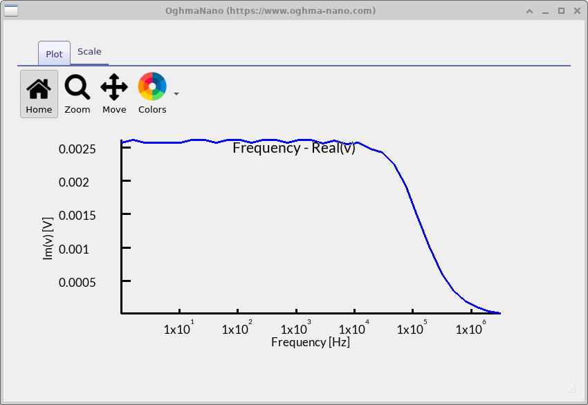
fx_real.csv — Bode (real) (??): Background: the real part is the in-phase photovoltage, i.e., the portion that rises and falls with the light without delay. Interpretation for this device: the curve shows a stable low-frequency plateau around \(\sim 2.5\ \text{mV}\), meaning the quasi-static \(V_\mathrm{oc}\) closely tracks the light modulation. Above roughly \(10^5\)–\(3\times10^5\ \text{Hz}\) the response rolls off toward zero, indicating the device can no longer sustain the photovoltage at rapid modulation—consistent with limited recombination lifetime and RC bandwidth.
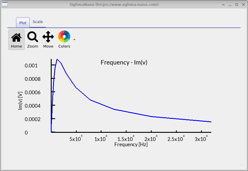
fx_imag.csv — Bode (imag) (??): Background: the imaginary part is the out-of-phase photovoltage and peaks where the system stores/release charge most strongly. Interpretation: a clear maximum appears around \(1.2\!\times\!10^5\)–\(2.0\!\times\!10^5\ \text{Hz}\). The peak frequency estimates the effective carrier lifetime via \(\tau \approx 1/(2\pi f_\text{peak})\), giving \(\tau \approx 0.8\text{–}1.3\ \mu\text{s}\). The moderate peak height suggests a single dominant recombination pathway rather than multiple overlapping processes.
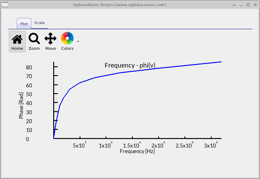
fx_phi.csv — Bode (phase) (??): Background: phase indicates how far the voltage lags the light modulation (0° = purely resistive/instantaneous; larger angles = more capacitive/slow). Interpretation: the phase climbs from near 0° at low frequency toward ~\(80^\circ\) in the 0.1–3 MHz range, matching the frequency band where the imaginary part is large. This confirms a strongly capacitive, lifetime-limited response near the IMVS peak.
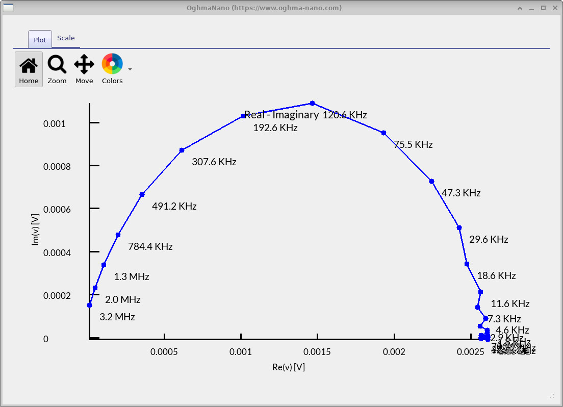
real_imag.csv — Nyquist (??): Background: plotting −Im(V) versus Re(V) maps the same dynamics into the complex plane; a semicircle typically indicates an RC-like process. Interpretation: the plot shows a single, well-formed semicircle with its apex labelled around \(120\text{–}200\ \text{kHz}\). The right-hand intercept (low-frequency limit) corresponds to the quasi-static photovoltage swing, while the left-hand intercept (high-frequency limit) tends toward zero as the device cannot build up voltage quickly. The single arc corroborates the \(\sim 1\ \mu\text{s}\) lifetime inferred from the Bode plots.

Overall, these IMVS results indicate a device that tracks light modulation well at low frequency, then transitions to a lifetime-limited regime with a characteristic timescale of roughly \(1\ \mu\text{s}\) near \(10^5\)–\(2\times10^5\ \text{Hz}\). The consistency between the real/imaginary Bode plots, the phase rise, and the Nyquist semicircle points to a single dominant recombination process setting the dynamic limit of the open-circuit photovoltage.

Below is a quick reference for the IMVS output files and what each one represents.

Filename	What it contains
`fx_real.csv`	In-phase (real) photovoltage vs. frequency, i.e., \(\mathrm{Re}[V(f)]\).
`fx_imag.csv`	Out-of-phase (imaginary) photovoltage, \(\mathrm{Im}[V(f)]\); the peak indicates the dominant lifetime.
`fx_phi.csv`	Phase of the IMVS response, \(\phi(f)\), showing how \(V\) lags the light modulation.
`real_imag.csv`	Nyquist view of photovoltage: −Im(V) vs. Re(V) with frequency markers along the arc.
`fx_abs.csv`	Magnitude \(\|V(f)\|\) of the IMVS response (absolute photovoltage).
`fx_C.csv`	Small-signal (differential) capacitance spectrum derived from the modulation analysis.
`fx_R.csv`	Effective differential resistance versus frequency, useful for RC time-constant estimates.

📝 Check your understanding (IMVS)

What does the low-frequency plateau in the Bode (real) plot reveal about how the device maintains its open-circuit voltage under steady illumination?
How can the peak in the Bode (imag) spectrum be related to the characteristic carrier lifetime or recombination rate?
Why does the Bode (phase) curve shift toward positive angles at higher frequencies, and what does this indicate about delayed voltage response?
What does the semicircle in the Nyquist plot represent, and how can its diameter and position be linked to recombination dynamics?
How would increasing or decreasing the light intensity affect the IMVS response, and what physical processes drive these changes?

💡 Tasks: Explore how IMVS responds under different physical and operating conditions:

Parasitic resistances: In the Electrical ribbon, open the Parasitic components editor. Increase the shunt resistance to a very high value (e.g. \(10^{12}\ \Omega\)), then reduce it to 100 Ω or 10 Ω, and rerun the IMVS simulation.
Carrier mobilities: In the Electrical parameters editor of the device structure, change the electron and hole mobilities. Try increasing them by two orders of magnitude and note the effect on the IMVS spectra.
Illumination intensity: In the Optical tab, switch the light level from 1 sun to dark. Compare the IMVS results under both conditions.

✅ Expected results

Shunt resistance: A high shunt resistance suppresses leakage, giving well-defined Nyquist semicircles. With a low shunt resistance (100 Ω or 10 Ω), leakage paths flatten the arcs and reduce the overall photovoltage amplitude.
Carrier mobilities: Higher mobilities speed up carrier extraction, shifting the IMVS peak to higher frequencies. For example, if the imaginary peak moves from \(1\times10^5\ \text{Hz}\) to \(3\times10^5\ \text{Hz}\), the inferred lifetime shortens from \(\tau \approx 1.6\ \mu\text{s}\) to \(\tau \approx 0.5\ \mu\text{s}\). Lower mobilities do the opposite: peaks shift to lower frequency, implying slower response.
Illumination: In the dark, there is no measurable IMVS response (no photovoltage). Under 1 sun, strong arcs appear: the peak frequency gives the recombination lifetime, typically in the range of \(0.5\)–\(2\ \mu\text{s}\) for OPVs. Shifting illumination intensity can also change arc size, reflecting different recombination dynamics.

6. Summary & next steps

In this tutorial you set up and ran IMVS (Intensity-Modulated Photovoltage Spectroscopy) in OghmaNano—exciting with Light, measuring Voltage, using a small modulation depth, and operating under open-circuit conditions. You learned how to read Bode and Nyquist plots of the photovoltage response: the low-frequency plateau shows that \(V_\mathrm{oc}\) tracks the illumination; the mid-frequency peak (and the Nyquist semicircle apex) identifies the dominant kinetic timescale, with \(\tau \approx 1/(2\pi f_\text{peak})\); and the high-frequency roll-off reflects the device’s RC/transport bandwidth. The same workflow applies to OPVs, perovskites, tandems, photodetectors, and LEDs whenever open-circuit photovoltage dynamics are of interest. For deeper analysis, export the CSV files (fx_real.csv, fx_imag.csv, fx_phi.csv, real_imag.csv) to extract lifetimes, fit equivalent-circuit or kinetic models, benchmark against experiment, and cross-check with IMPS/IS to separate recombination from collection and contact effects.