Ray-tracing Tutorial (Part B): Editing light sources
In Part A you loaded the Reflection from film ray-tracing demo and inspected how rays reflect from a rough surface derived from an AFM image. In this part you will learn how to edit the light sources: changing their position, orientation and emission pattern, and then re-running the simulation to see how the reflected rays respond.
Step 1: Open the light editor
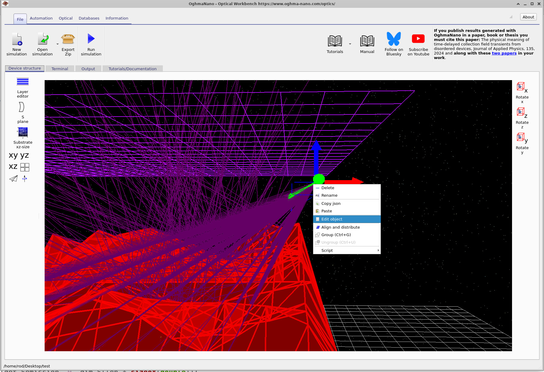
Start from the simulation you created in Part A. Rotate and zoom the view so that you can clearly see one of the green light source markers. Then right-click on the light source and choose Edit object from the context menu, as shown in ??. This opens the light source editor window.
Here you control the position (Offset), physical size (xyz size) and rotation of the emitting patch. With zero rotation, dx and dy define a flat rectangular source aligned with the x and y axes.
Step 2: Set the position and size (Object tab)
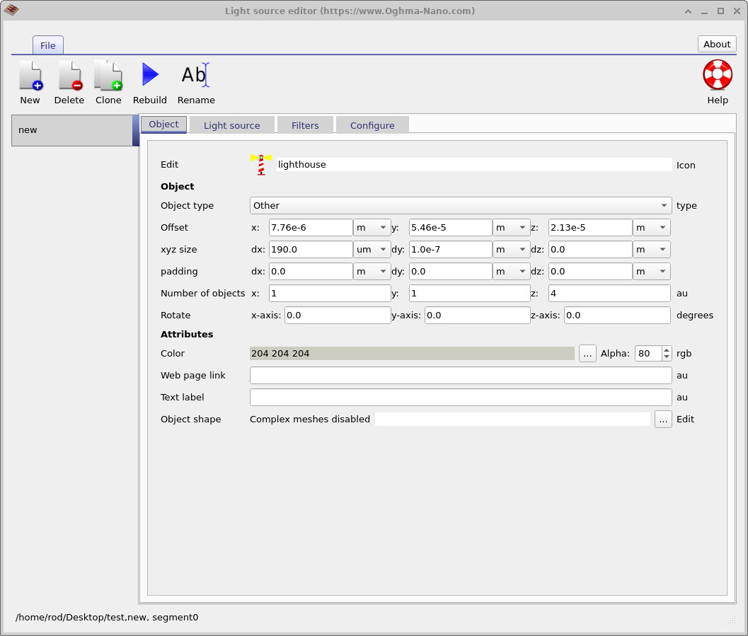
The light source editor opens on the Object tab (??). This tab is common to many object types in the Optical Workbench. It controls:
- Offset (x, y, z): the position of the object in 3D space.
- xyz size (dx, dy, dz): the physical size of the object along each axis.
- Rotate: rotation around the x, y and z axes.
- Number of objects: how many copies of the object are created in x, y, z.
For our light source, the important values are dx and dy, which specify the width and height of the emitting region in the x–y plane. When the rotations are set to zero, this corresponds to a flat, rectangular patch that is aligned with the grid. This patch is then used as the starting area from which individual beams are launched.
For now, leave the position and size unchanged. In later parts of the tutorial you can experiment with making the source larger or smaller, or creating multiple sources using the Number of objects fields.
Step 3: Control emission angles (Configure tab)
Next, click the Configure tab of the editor. This displays settings that determine how the source emits light, as shown in ??.

The key fields are:
-
Illuminate from: set to
xyzin this example, meaning the light source is positioned in 3D space and can be moved freely using the Offset entries on the Object tab. - Rotate Theta (θ): the polar angle that sets the main pointing direction of the beams, measured from the positive z-axis.
- Rotate Phi (φ): the azimuthal angle around the z-axis, measured in the x–y plane.
- −Δθ, +Δθ and −Δφ, +Δφ: the angular ranges around the central (θ, φ) direction through which the source scans. In this demo there is one step in θ and ten steps in φ, so the beams sweep out a fan in the azimuthal direction.
-
Number of beams x / y: how many independent rays are launched across
the emitting patch in the x and y directions. For example,
Number of beams x = 30means 30 distinct beam positions along the x-axis.
In the configuration shown, θ is set to 0°, so the main direction of emission is horizontal, while φ = 30° means the fan of beams is rotated in the x–y plane. The scanning steps in φ cause the light to sweep sideways across the detector.
Step 4: Understanding θ and φ in the 3D view
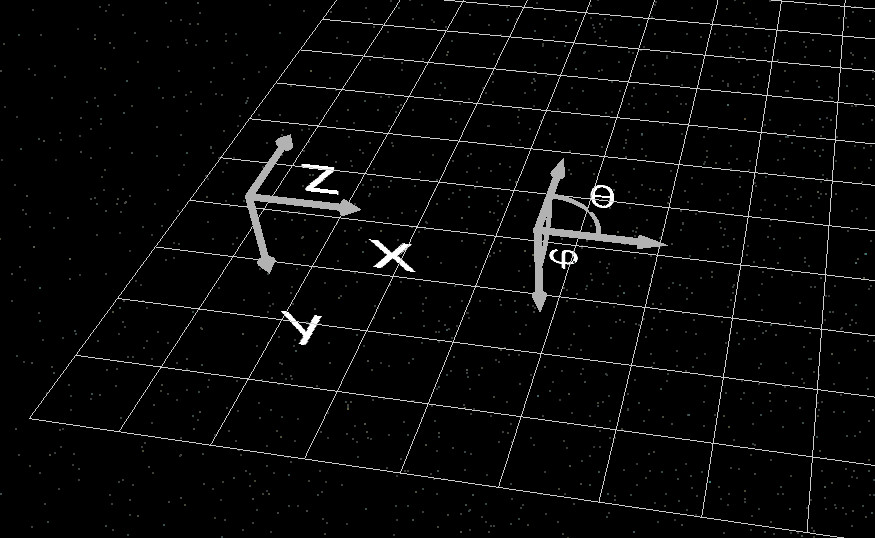
You might reasonably ask: how do I know which way θ and φ point? To help with this, the Optical Workbench displays small orientation markers in one corner of the simulation window, as illustrated in ??. These show the x, y, z axes and the definitions of θ and φ.
If the markers are not immediately visible, rotate or zoom the view slightly; they are always located near one of the corners of the 3D scene.
Step 5: Point the beams downwards
As an exercise, you will now re-orient the light source so that it points downwards onto the rough film instead of sideways.
- In the Configure tab, adjust Rotate Theta and Rotate Phi so that the main beam direction is towards the film.
- Keep the ranges (−Δθ, +Δθ, −Δφ, +Δφ) and the number of beams unchanged for now.
- Click Rebuild in the light editor toolbar to apply the changes.
- Close the editor and click Run simulation (or press F9) to re-run the ray tracing.
You should see the rays now strike the surface from above rather than sweeping in from the side. Comparing the new ray pattern with the original configuration is a good way to build intuition for the θ and φ angles.
Step 6: Move the light source in 3D
Once you have a downward-pointing source, you can also move it laterally to illuminate different regions of the rough film. In the main 3D view, select the light source and drag it with the left mouse button to a new position near the centre of the surface. An example is shown in ??.
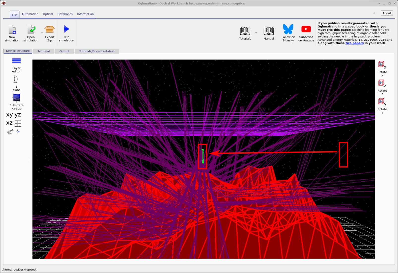
After moving the source, run the simulation again and observe how the distribution of rays on the detector changes. You can also inspect the updated detector efficiency curves in the Output tab, as described in Part A.
A final note on optical sources
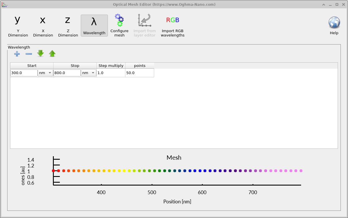
The number of wavelengths emitted by a light source is controlled from the Optical ribbon using the Optical Mesh Editor (??). The mesh defines the spectral sampling used during the ray-tracing calculation, and it has a direct impact on both the accuracy of wavelength-dependent plots (for example reflection or transmission spectra) and the overall simulation speed.
As a general rule, it is best to begin with a small number of wavelengths while setting up a simulation. A coarse mesh of around 8 wavelengths is usually sufficient for positioning light sources, checking geometry, and verifying that rays behave as expected. Once you are confident that the configuration is correct, you can increase the mesh density to 40–50 wavelengths to obtain smooth, high-quality optical spectra.
Each wavelength is simulated independently on a separate CPU thread. This means that if your computer has many cores, OghmaNano will scale almost linearly with the number of wavelengths: more available threads lead to faster multi-wavelength simulations. Conversely, choosing an excessively fine mesh on a machine with only a few cores may slow the simulation down noticeably. Selecting an appropriate number of wavelengths is therefore a balance between accuracy and speed.
👉 Next step: Continue to Part C to explore more advanced analysis, including angle-resolved statistics and exporting data for external plotting. For an overview of optical systems and ray-tracing simulations, see Optical systems and ray tracing overview.