Ray-tracing Tutorial (Part A): Reflection from a Rough Film
In this tutorial you will use OghmaNano’s ray tracer to study how light reflects from a rough film. The roughness can represent an AFM image or any other experimentally measured surface. You will load the Reflection from film demo, run a ray-tracing simulation, and examine how efficiently light is captured by a detector above the film.
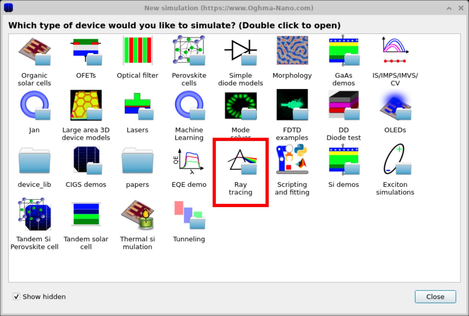
Step 1: Open the ray-tracing examples
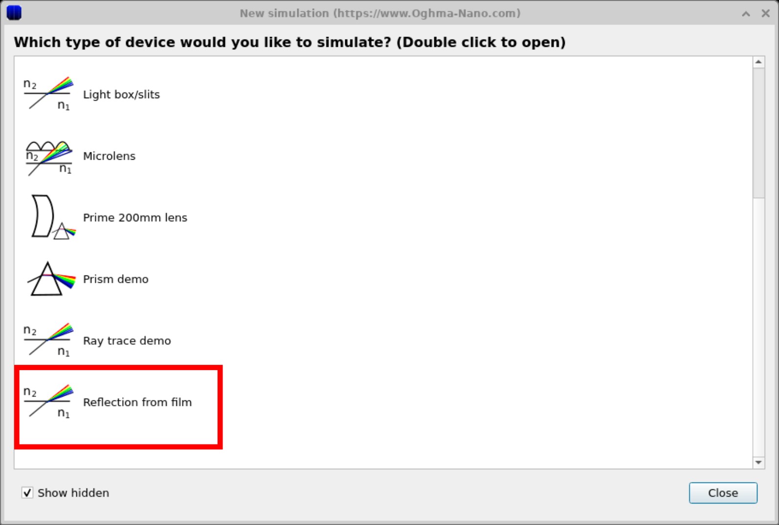
Launch OghmaNano from the Windows Start menu. From the start window, click New simulation. This opens the device-type library. Locate and double-click the Ray tracing category as shown in ??. This will open the folder of ray-tracing demos (??).
When prompted, choose a directory where the simulation should be saved. As with all OghmaNano simulations,
it is best to use a local folder (for example on C:\) rather than a network or cloud drive. You can read more about simulation speed here.
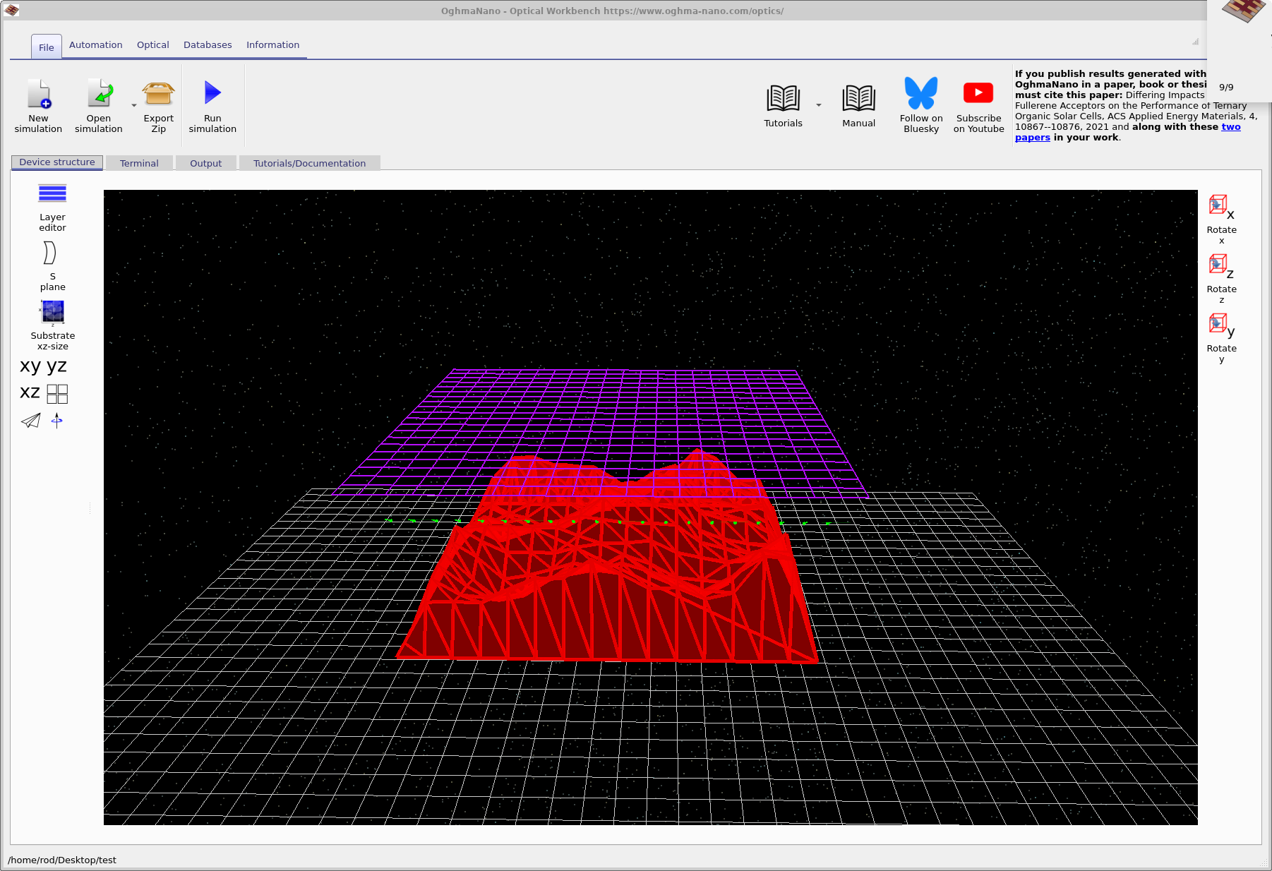
Step 2: Inspect the film and detector
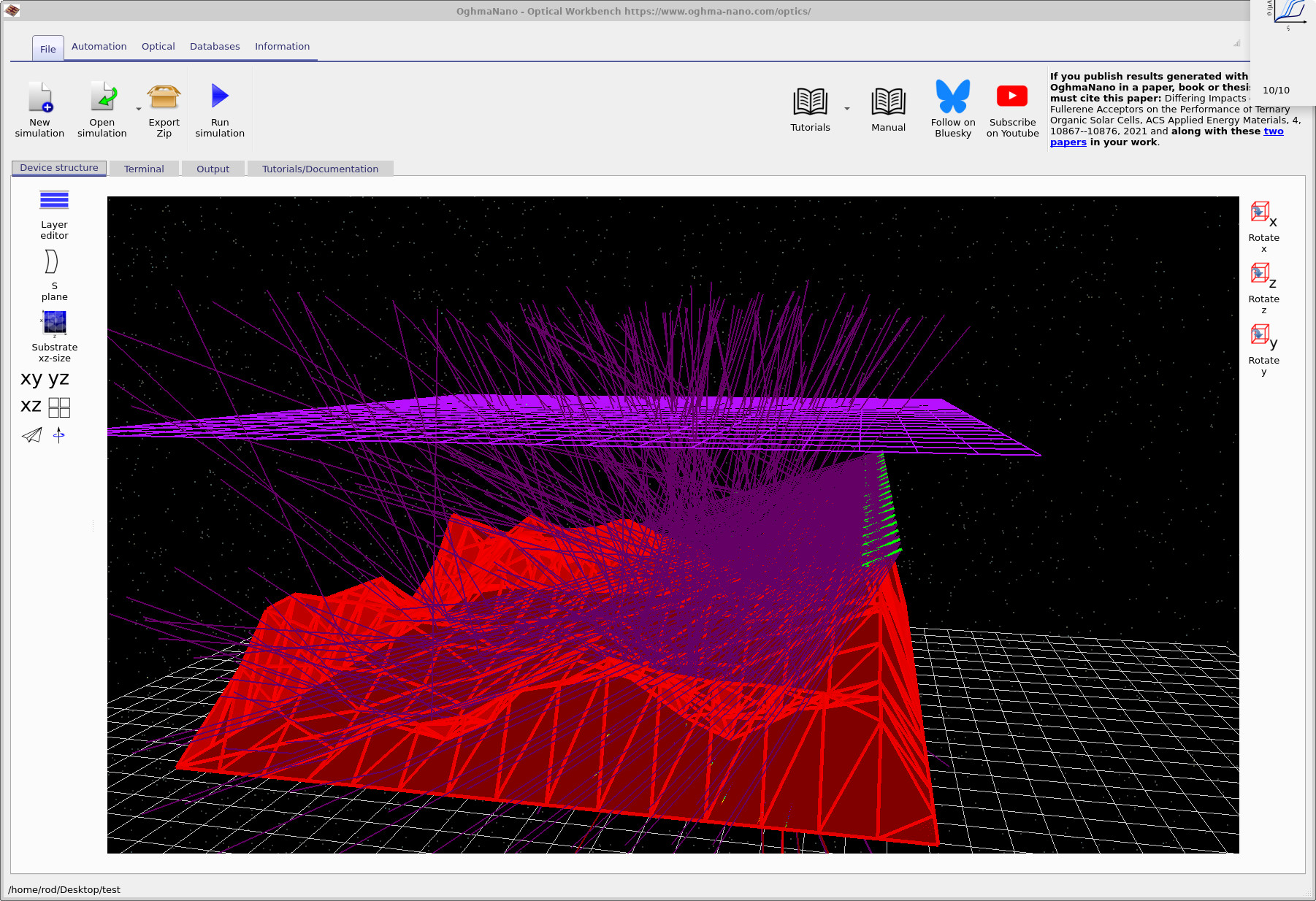
After selecting Reflection from film, the main Optical Workbench window opens and shows the 3D scene (??). The red surface represents the rough film (for example, an AFM height map), the green arrows are the light sources, and the purple grid above the film is the optical detector – conceptually similar to a CCD camera.
You can navigate the 3D view using the mouse:
- Left mouse button: rotate the scene.
- Right mouse button: pan the view.
- Mouse wheel: zoom in and out.
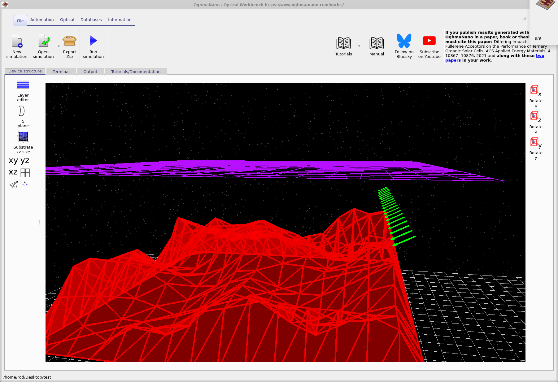
Step 3: Run the ray-tracing simulation
To start the simulation, click the Run simulation button (blue play icon) in the toolbar or press F9. OghmaNano will trace many rays from the sources, reflecting and refracting them according to the local surface normal of the film. As the simulation runs, the main view will update to show the paths of the rays (??).
Step 4: Explore different wavelengths
The Wavelengths widget in the Optical ribbon lets you choose which wavelength is currently visualised in the 3D view. Select a wavelength from the drop-down box as shown in ??. This does not rerun the simulation – the full spectrum is precomputed – but it controls which subset of rays is displayed.
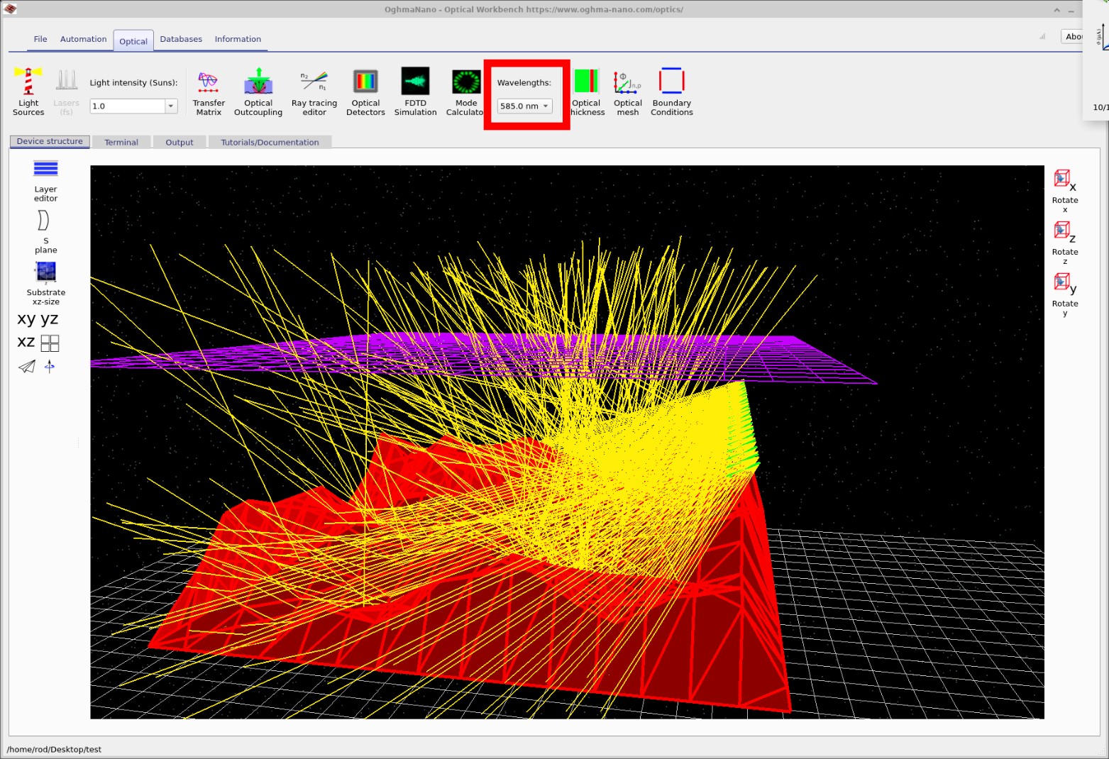
Try a few wavelengths and observe how the ray density at the detector changes. In later parts of the tutorial you will see how this relates to interference, scattering and absorption in the film.
Step 5: View the detector output
When the ray tracing is complete, switch to the Output tab to view the files written to disk (??). You will see a range of files describing the rays and detector responses. The most relevant for this tutorial is the detector0 directory, which contains the data recorded by the purple detector plane.
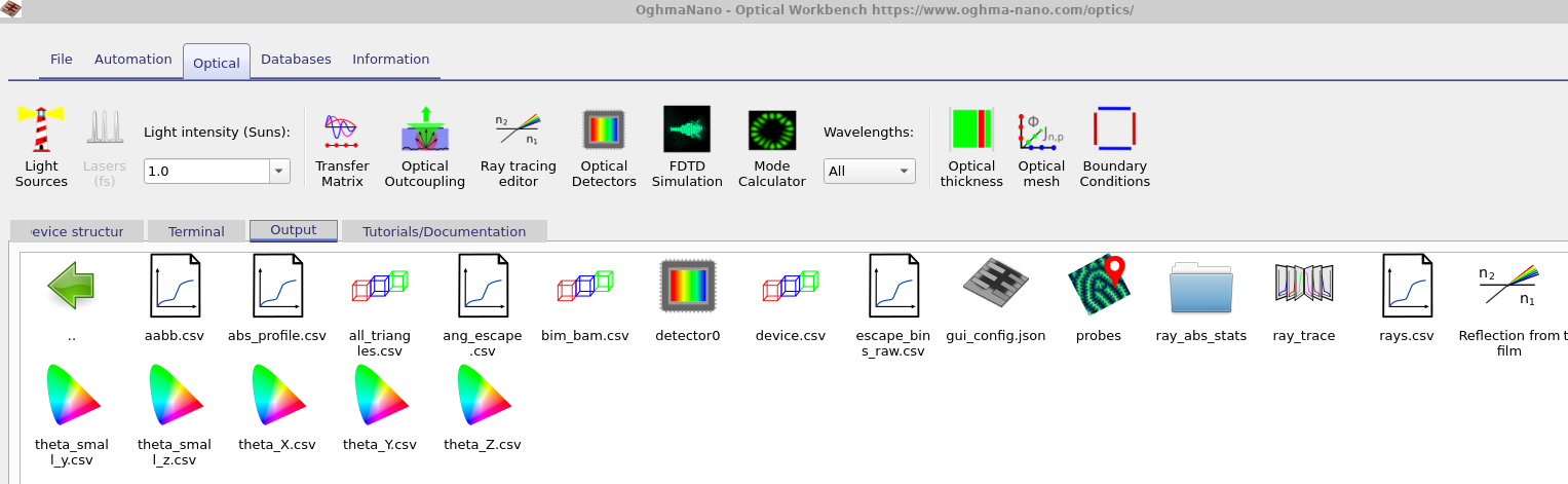
detector0 folder contains the response of the detector plane; other files describe the individual rays and angular distributions.
Double-click the detector0 folder, then open the file
detector_efficiency0.csv.
This file stores the fraction of light energy arriving at the detector as a function of wavelength.
When you open it, OghmaNano’s plotting tool will show a spectrum similar to
??.
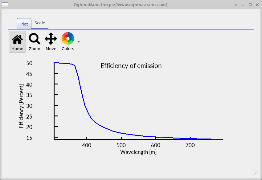
detector_efficiency0.csv.
The vertical axis shows the fraction of light that reaches the detector. When a ray leaves the source it has intensity 1;
attenuation and scattering by the rough film reduce this value before it reaches the detector.
In this example almost no light is detected at long wavelengths, while shorter wavelengths are captured more efficiently.
(The axis label currently shows metres, but the horizontal axis should be interpreted as wavelength in nanometres.)
By comparing the detector efficiency curve to the visualised rays at different wavelengths, you can build intuition for how surface roughness, scattering and angular distribution affect the detected signal.
The output files from your simulation
Each ray-tracing simulation generates a collection of files that describe the geometry, the individual rays, and the response of any detectors.
Most of these are plain .csv files that can be opened in OghmaNano’s built-in viewers or analysed in external tools such as Python, Matlab or Excel.
The key outputs for the Reflection from film demo are summarised in Table 1.
| File or folder | Description |
|---|---|
| rays.csv | List of traced rays (positions, directions, wavelengths, and intensities). |
| ray_trace/ | Additional ray-trace diagnostics and statistics. |
| detector0/detector_efficiency0.csv | Detector efficiency vs wavelength (see ??). |
| detector0/detector_input0.csv | Total light incident on the detector plane vs wavelength. |
| RAY_image.csv | Image-like representation of rays on the detector plane. |
| device.csv | Geometric description of the rough film and detector surfaces. |
👉 Next step: Continue to Part B to learn how to modify the rough surface, adjust the light sources, and run parameter sweeps. For an overview of optical systems and ray-tracing simulations, see Optical systems and ray tracing overview.