Chapter 4: Optical systems & ray tracing

1. Introduction

This chapter introduces ray tracing in OghmaNano for modelling optical systems using geometric optics. It explains the fundamental principles of physics-based ray tracing and how they are applied to simulate light propagation, optical components, and system-level performance.

There are two fundamentally different ways of describing light: as a wave and as a particle. In principle these descriptions are unified by quantum mechanics, but in practice, when modelling optical systems for physics or engineering applications, one must usually choose which description is appropriate for the problem at hand.

Wave-based optical methods are required when the characteristic size of a structure is comparable to the wavelength of light, such as in thin-film solar cells or nanostructured materials (e.g. thin films). In this regime, phase, coherence, interference, diffraction, and electromagnetic field propagation become important, so numerical techniques such as finite-difference time-domain (FDTD) or transfer-matrix methods are often needed. When the structure is much larger than the wavelength, these wave effects are usually less important, and simpler geometric ray-tracing models are typically sufficient.

When the characteristic size of a system is much larger than the wavelength of light (e.g. in lens systems), light can be accurately modelled as rays. This is the basis of geometric optics and the focus of this chapter. Rays carry position, direction, wavelength, and intensity, and interact with surfaces through refraction, reflection, absorption, and clipping, enabling efficient modelling of complete optical systems.

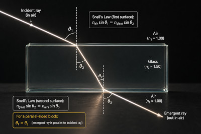
At the heart of ray tracing is Snell’s law, which determines how light refracts at an interface between two materials:

\[ n_1 \sin(\theta_1) = n_2 \sin(\theta_2) \]

This relation governs how rays bend when crossing boundaries between materials with different refractive indices. It also underpins phenomena such as total internal reflection. An example of refraction through a simple optical element is shown in ??.

When designing optical systems, Snell’s law is applied repeatedly at every interface, allowing rays to be traced through complex assemblies of lenses and surfaces. A full system-level example is shown in ??, where rays propagate through a multi-element lens before reaching a detector.

In practical implementations, ray tracing is performed in three dimensions. This requires a vector form of Snell’s law, where the incident ray direction, transmitted ray direction, and surface normal are treated explicitly as vectors:

\[ \mathbf{k}_t = \frac{n_1}{n_2}\mathbf{k}_i + \left(\frac{n_1}{n_2}\cos\theta_i - \cos\theta_t\right)\mathbf{n} \]

In addition to refraction, a complete optical model must also account for reflection and transmission at interfaces. These are governed by the Fresnel equations, for example: \[ R = \left|\frac{n_1 \cos\theta_i - n_2 \cos\theta_t}{n_1 \cos\theta_i + n_2 \cos\theta_t}\right|^2, \quad T = 1 - R \] which determine how much optical power is reflected or transmitted at each boundary.

By combining refraction (Snell’s law), reflection, and transmission at every interface, a complete physics-based ray-tracing framework can be constructed. While additional effects can be included, these form the fundamental building blocks of geometric optical simulation.

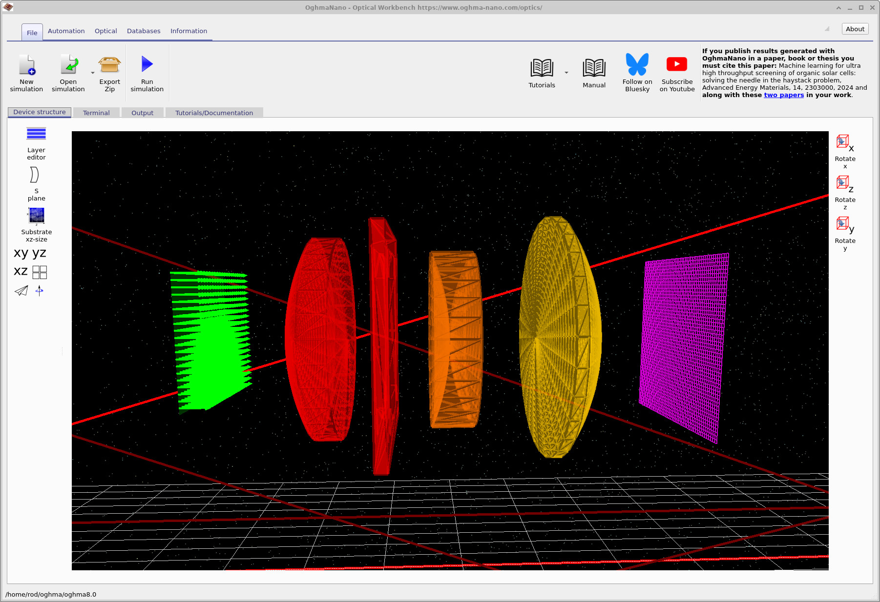
OghmaNano includes a highly efficient multi-threaded ray tracer for analysing optical systems and components. It is both spectral, allowing simulation across multiple wavelengths, and fully 3D, enabling accurate modelling of complex geometries and off-axis effects. The same framework is used throughout the optical tutorials: defining light sources, editing optical surfaces in the S-plane editor, evaluating lenses such as the modern 200 mm prime lens, running automated S-plane parameter scans, and using figures of merit to quantify optical performance.

Ray tracing is also useful beyond conventional lens design. OghmaNano can be used to study reflection from rough films, light escape from structured films, and microlens-based optical filtering, where surface shape, scattering, and collection geometry all affect the final optical response.

The pages below form a connected cluster. If you are new to OghmaNano, start with the overview, then move on to detectors, and finally work through a complete lens system as a worked example.