Cooke Triplet Lens Tutorial (Part B): Analysing Optical Performance

Exploring aberrations with a narrow beam

In Part A we traced a broad beam through the Cooke Triplet and confirmed that the system forms an image on the detector. In this section we switch to a small square source patch and a reduced ray count. This makes the detector output behave like a simple spot diagram: instead of a dense blur, you can clearly see the footprint of different rays and how that footprint changes as you move off-axis.

Two ideas to keep in mind as you work through this section:

• On-axis rays test how well the lens corrects “symmetric” aberrations such as spherical aberration and longitudinal chromatic focus shift.
• Off-axis rays (field points) reveal aberrations that grow rapidly with field angle, especially coma, astigmatism and lateral colour.

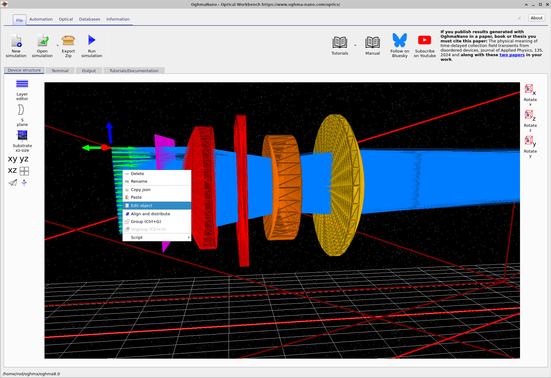
In the Device structure view, right-click on the green light source and choose Edit object, as shown in ??. This opens the Light source editor where we can control (i) the physical size of the emitting patch and (ii) how many rays are launched across that patch.

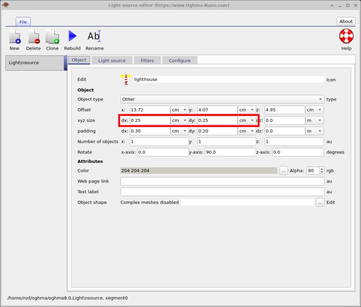
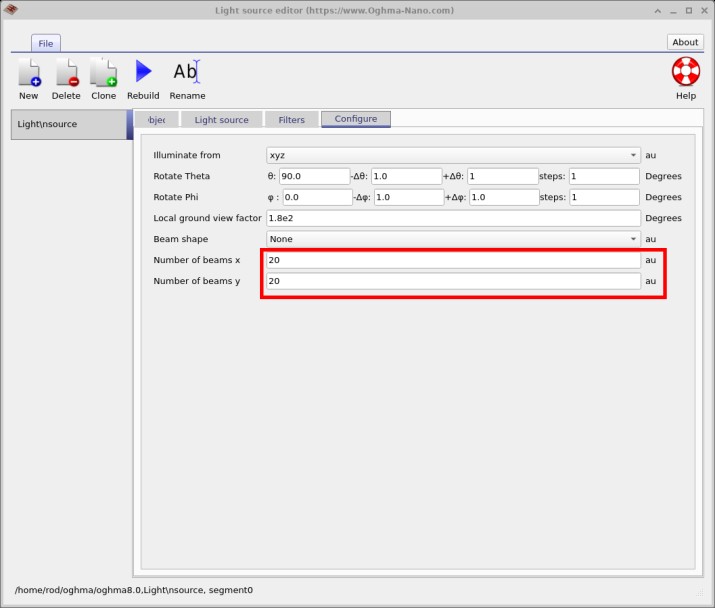
In the Object tab (??), set dx = 0.25 cm and dy = 0.25 cm. You can leave dz unchanged (the source is a 2D sheet in this setup).

Now switch to the Configure tab (??) and set Number of beams x = 20 and Number of beams y = 20. This gives a sparse but informative sampling: enough rays to show the shape of the spot, without turning it into a solid blob.

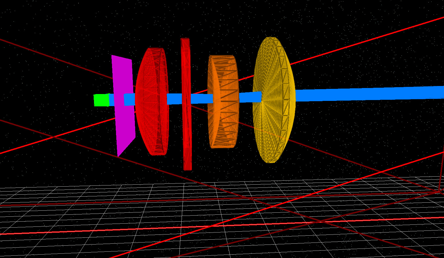
Close the editor and rotate the 3D view so you can see the source, the three lenses, and the detector in one line. Position the light source so the narrow beam enters the centre of the first (red) element, as shown in ??.

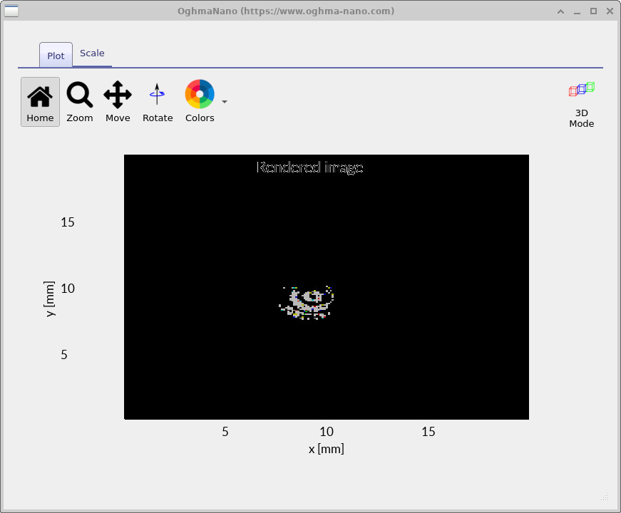
Click Run simulation, then open the Output tab, navigate to detector0, and open RAY_image.csv to view the on-axis spot diagram (??).

On-axis, the footprint is small and fairly symmetric. In your rendered image you can already read a few useful things:

• Spot size: the cluster is not a single pixel, so the detector is not exactly at the “perfect” focal plane for all rays. Some spread is expected because you are sampling a finite patch and because real designs retain residual higher-order aberrations.
• Shape: the spot is approximately round rather than strongly elongated. That is what you want on-axis: large asymmetries on-axis would usually indicate misalignment, strong coma (unexpected here), or a detector plane placed very far from best focus.
• Chromatic behaviour: the coloured speckles are close together but not perfectly coincident. This is the visible signature of chromatic focus shift: different wavelengths are being brought to slightly different axial focus positions, so at a fixed detector plane you see small colour fringing within the spot.

Off-axis aberrations: field shift, coma and astigmatism

Next we deliberately move the source off-axis to probe field performance. This is where classic photographic aberrations become obvious: the “centre of the image” is usually sharp, while points towards the edge acquire asymmetric blur.

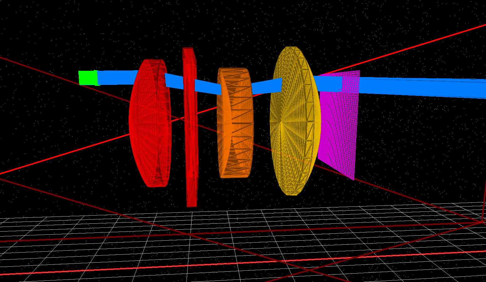
In the 3D view, drag the light source upward so it no longer illuminates the centre of the first lens, as shown in ??. Keep the beam direction roughly the same; we want an off-axis field point, not a different pointing direction.

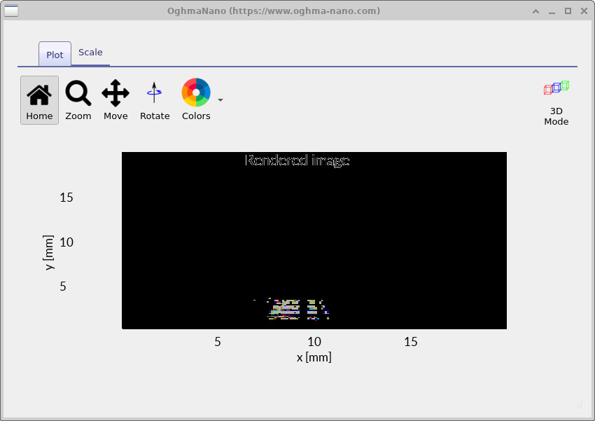
Run the simulation again and reopen RAY_image.csv in detector0 (??).

Compared with the on-axis result, three changes should jump out immediately:

• Field shift: the spot is no longer centred in the detector image. Even if the lens forms a sharp image, an off-axis field point maps to a different position on the detector. This displacement is expected and is part of normal imaging geometry.
• Coma (asymmetry): the footprint becomes noticeably one-sided rather than round. In practical terms, coma means different pupil zones “miss” the ideal image point by different amounts, so the spot gains a bright core plus a smeared, directional halo instead of a symmetric blur.
• Astigmatism / field curvature (directional spread): the off-axis spot is stretched more strongly along one direction. This is the usual sign that tangential and sagittal ray bundles would prefer different best-focus planes. At the fixed detector plane, one direction appears closer to focus while the orthogonal direction is still defocused.

You can also see that the colour separation is larger off-axis. This is lateral chromatic aberration: different wavelengths land at slightly different lateral positions in the image plane, which shows up as coloured streaking within the spot. In a well-corrected photographic lens this is controlled (not eliminated), and it typically becomes more noticeable towards the edge of the field.

The key takeaway is that the Cooke Triplet is behaving like a real historical photographic design: good central performance, and then a progressive increase in coma/astigmatism/colour errors as you move off-axis. This is exactly what makes it a useful teaching example: you can see the “textbook” aberrations appear with only a simple source shift.