Figures of Merit (Part A): Evaluating Ray-Traced Optical Performance in OghmaNano
1. Introduction
Ray tracing can produce a large volume of visual output—ray bundles, detector images, and 3D geometry-but "looks good" is not a design criterion. In this tutorial we focus on figures of merit (FoM): quantitative metrics that compress a detector image and ray-trace statistics into well-defined numbers that can be compared, ranked, and interpreted.
In this tutorial, we examine how these figures of merit are generated for an individual optical system and what they physically represent. We extract and interpret common metrics including spot size (σx, σy), RMS spot radius, major and minor axis spot radii, spot ellipticity and spot orientation angle, encircled energy radii (EE50, EE80, EE90, EE95, EE99), halo energy fraction, and energy concentration ratios. The emphasis is on understanding how each metric is constructed, when it is useful, and which aspects of optical performance it captures—or obscures.
Once these figures of merit are understood at the single-design level, they can be applied systematically. The same metrics are used directly by OghmaNano’s parameter scan tool to track optical performance across design space and to drive optimisation. This tutorial therefore establishes the conceptual foundation for evaluating optical performance, while the accompanying scan tutorial demonstrates how to apply these figures of merit at scale.
cting2. Open the Cooke triplet example
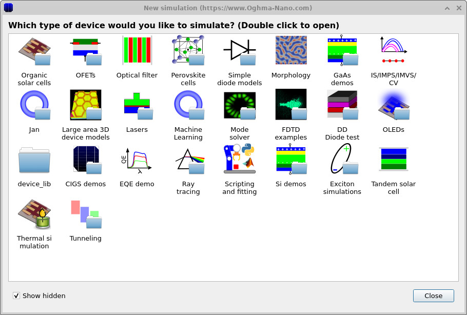
We will start from a preconfigured ray-tracing example so that you can focus on evaluating figures of merit rather than building an optical model from scratch. Begin by starting OghmaNano from the Windows Start menu. In the main window, click the New simulation button to open the simulation library, shown in Figures 2a–b.
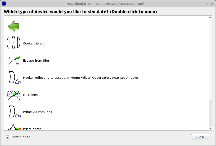
From the list of device categories, double-click Ray tracing to open the S-plane optics demos. From this list, explicitly select and open the Cooke triplet example. This classical multi-element lens provides a deliberately imperfect but well-behaved optical system, making it ideal for demonstrating how different figures of merit respond to changes in optical design.
💡 Tip: Save the simulation to a local drive such as
C:\. Even when you focus on FoM, scans and optimisers still produce CSV outputs and (optionally) ray/mesh files.
Network, USB, or cloud-synced folders can become I/O-limited and run
substantially more slowly.
3. Inspect the optical system and identify where figures of merit come from
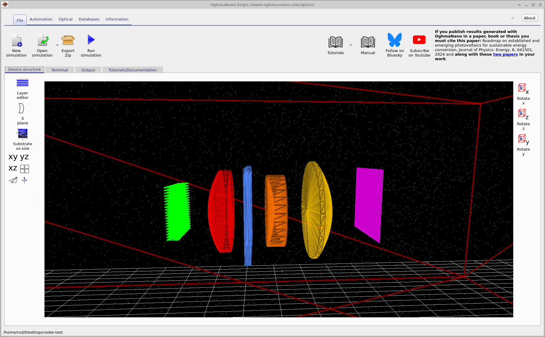
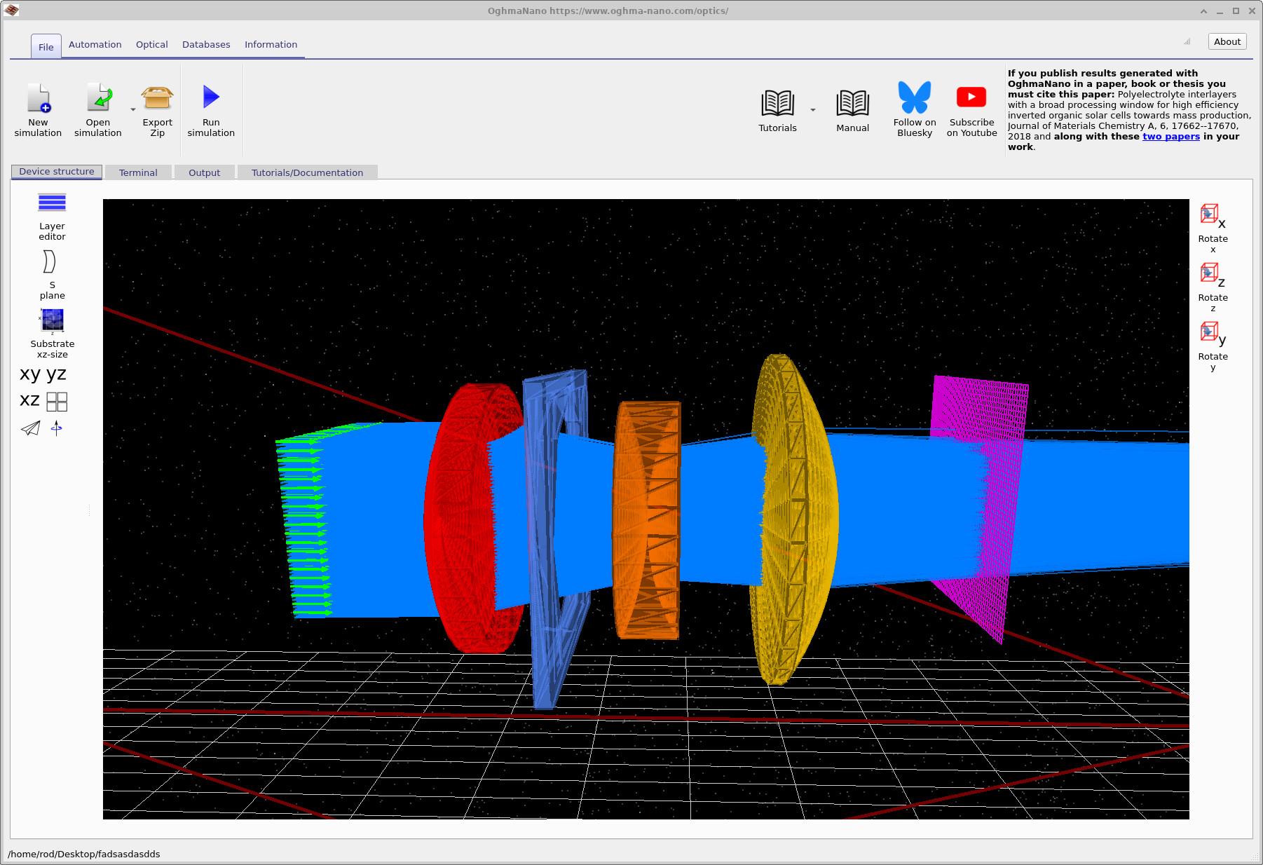
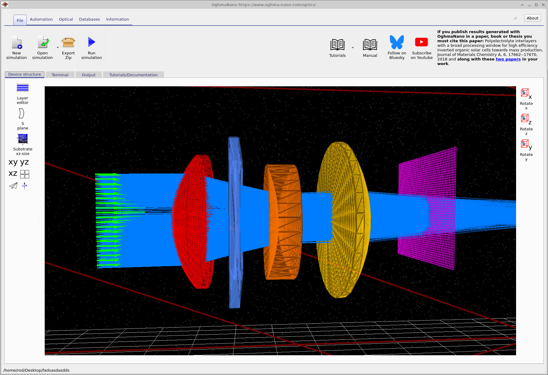
After opening the example, the main window should look like ??. The 3D view shows the complete optical system from source to detector. From left to right, the green arrows indicate the incident light rays emitted by the source. These rays first encounter the red optical element, which is the first lens of the system. The thin blue element that follows is the aperture stop, which limits the numerical aperture and controls which rays are allowed to propagate through the system.
Downstream of the aperture, the rays pass through the second lens (shown in orange) and then the third lens (shown in yellow). Together, these three refractive elements form a classic Cooke triplet: a historically important three-element lens design developed in the late 19th century, valued for its ability to correct spherical aberration, coma, and astigmatism using only simple spherical surfaces and common optical glasses. Variants of the Cooke triplet remain widely used today as the conceptual basis for many photographic and imaging lenses.
Finally, the rays intersect the detector plane, shown as a purple grid. All figures of merit are ultimately derived from the ray distribution on this plane. The spatial pattern of ray intersections is reduced to quantitative metrics such as centroids, spot radii, standard deviations, encircled-energy curves, and related measures of optical performance.
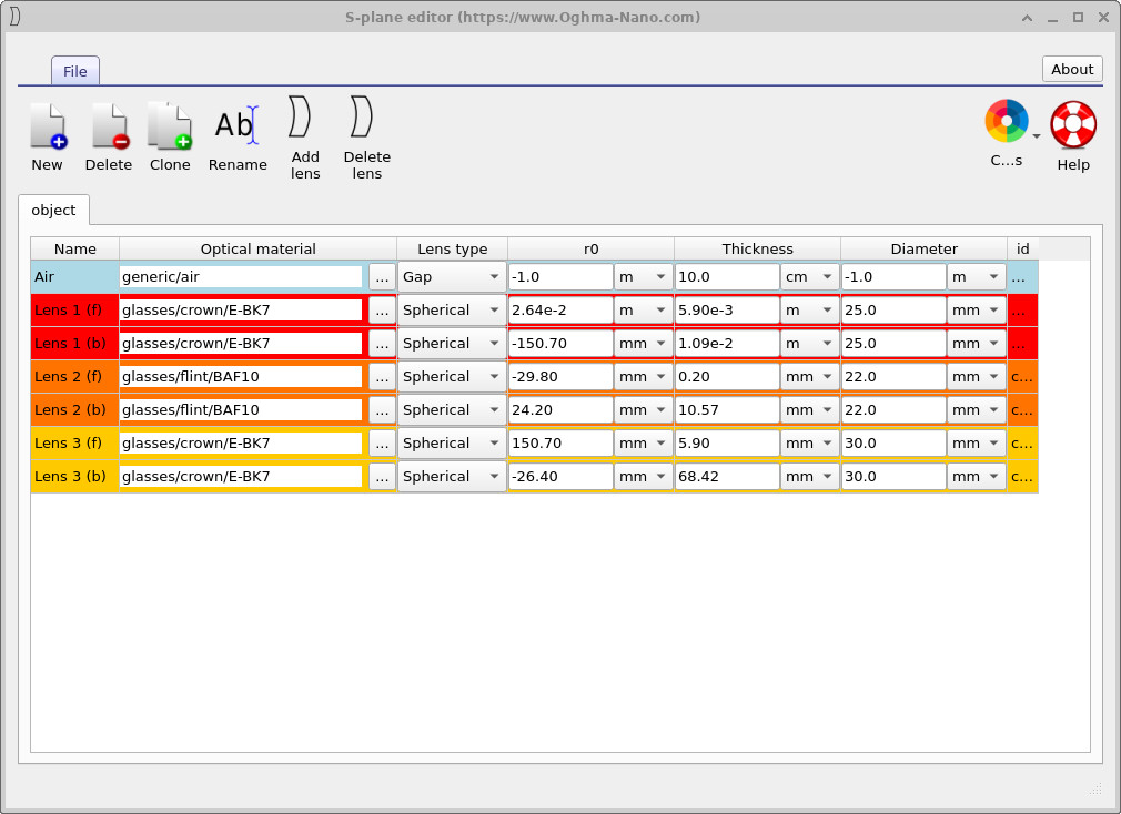
The same optical system is represented parametrically in the S-plane editor, which can be opened by clicking the S-plane button in the left toolbar, as shown in ??. Each row in the S-plane table corresponds directly to one physical surface in the 3D view, including the three lens elements and the aperture stop. In this tutorial you do not need to modify these parameters; their role here is to make clear which quantities define the system geometry and which parameters will later be varied when performing automated scans.
For a more detailed discussion of the Cooke triplet itself — including its optical layout, design philosophy, and historical background — see the dedicated tutorial Cooke Triplet Tutorial (Part A) .
4. Inspecting the simulation output and detector figures of merit
After running the simulation, the first confirmation that the system is behaving sensibly comes from inspecting the ray-trace itself (??). Here, rays emitted by the source are shown propagating through the three refractive elements of the Cooke triplet, being spatially filtered by the aperture stop, and finally intersecting the detector plane. This view is primarily qualitative: it allows the user to verify that rays are neither clipped unintentionally nor diverging catastrophically, and that the optical axis, element ordering, and aperture placement are consistent with expectations.
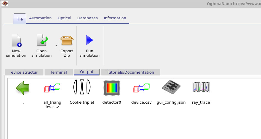
Quantitative analysis begins in the Output tab
(??),
which contains all files produced by the ray-tracing engine. The file device.csv
stores the full geometric description of the optical scene, including lens surfaces and
detector planes. The file all_triangles.csv contains the triangulated mesh used
internally for ray–surface intersection testing; visualising this file allows the user to
inspect the actual computational geometry rather than the idealised analytic surfaces.
The folder ray_trace provides a detailed representation of individual ray paths
through the system and is useful for diagnosing aberrations, vignetting, or unexpected ray
loss. The most important folder for performance analysis, however, is detector0.
Double-clicking this folder opens the detector output directory shown in
??.
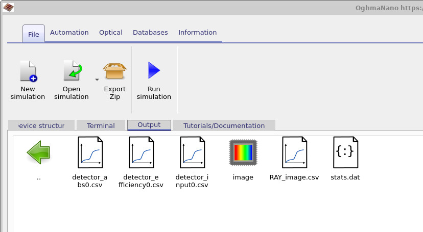
Within the detector directory, the file detector_abs_0.csv records the spatial
distribution of optical power absorbed by the detector surface. The file
detector_input.csv stores the total optical power launched into the system,
providing a reference against which all efficiencies are calculated. The file
detector_efficiency_0.csv contains the detector efficiency, defined as the
fraction of incident optical power that reaches the detector plane after propagation
through the optical system.
The detector directory contains two complementary ways to visualise what light reaches the image plane: a single RGB rendering that approximates what a colour-sensitive detector (for example, a CCD/CMOS camera) would “see”, and a wavelength-resolved snapshot viewer that allows the detector intensity distribution to be inspected as a function of wavelength.
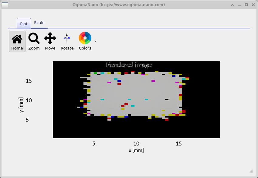
The file ray_image.csv stores the combined RGB detector image. Internally, this is constructed by
taking the full wavelength-dependent ray distribution produced by the simulation and mapping it into red,
green, and blue channels to form a single composite image. The result is an intuitive “camera-like” view of the
spot on the detector, combining all wavelengths into one colour image, and is useful for quickly diagnosing gross
chromatic effects, vignetting, and overall image placement.
Separately, the image directory provides a wavelength-resolved breakdown of detector illumination.
Double-clicking image opens the simulation snapshots viewer
(??).
This viewer is designed for inspecting how the detector-plane intensity distribution varies across the simulated
spectrum rather than collapsing everything into a single RGB composite.
In the snapshots viewer, use the + button to add data.csv to the file list. Once loaded,
the main plot shows the detector intensity at a particular wavelength (460 nm in the example shown), and the
wavelength slider beneath the plot allows you to step through the full propagated wavelength range to see how the
spatial distribution evolves. In effect, this provides a spectral “stack” of detector images: a direct way to
separate chromatic blur, chromatic focal shift, and wavelength-dependent vignetting from the visually appealing
but integrated RGB rendering.
For a fuller description of the snapshots system — including how snapshot datasets are organised on disk and how to use the viewer controls — see the dedicated page Output snapshots.
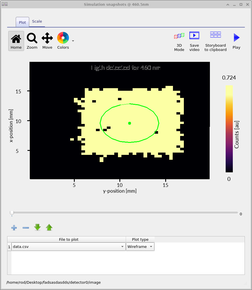
data.csv, the plot shows the
wavelength-resolved detector intensity (460 nm here). The slider steps through wavelength to inspect
chromatic variation in the detector-plane intensity distribution.
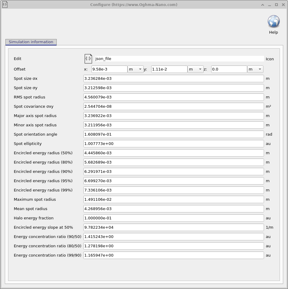
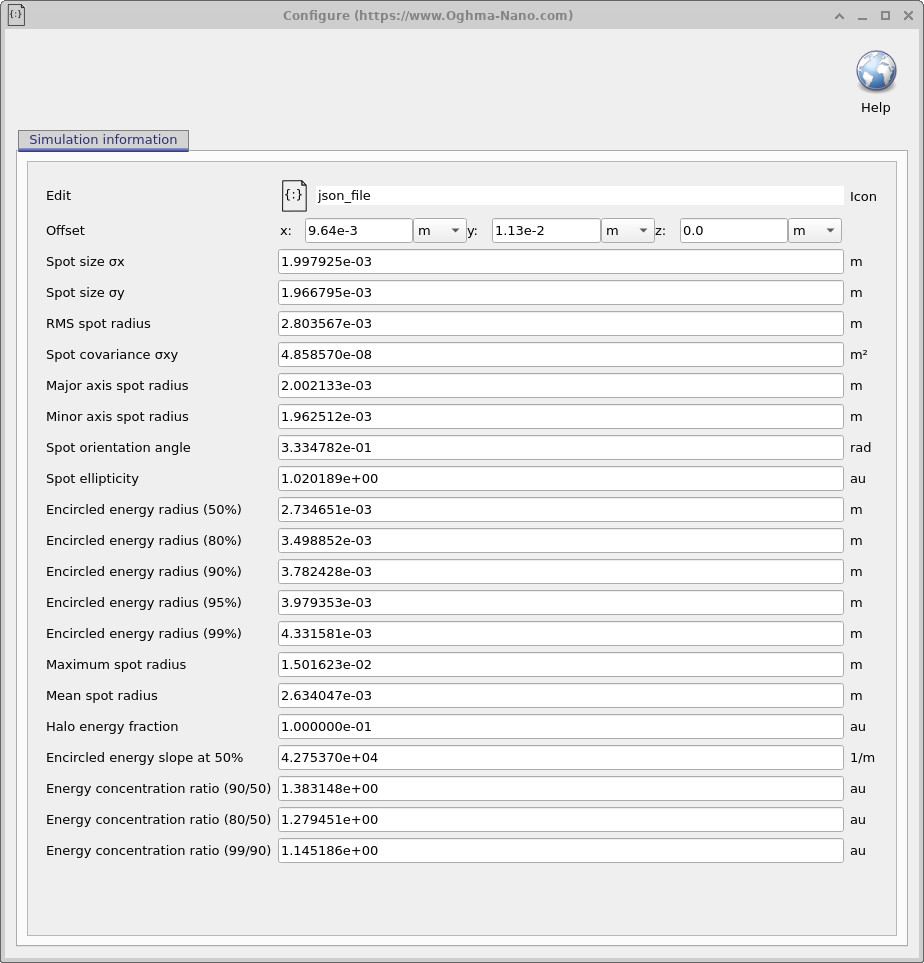
The most important output for quantitative analysis is stats.dat, which opens
the detector statistics window shown in
??.
This window lists all figures of merit derived from the ray distribution on the detector plane.
These metrics provide an objective, reproducible basis for comparing optical designs,
optimising parameters, and performing automated scans.
| Metric | Symbol / Definition | Physical meaning and interpretation |
|---|---|---|
| Offset (x, y, z) | \((x_0, y_0, z_0)\) | The spatial offset of the detector plane relative to the nominal optical axis. Non-zero offsets indicate image shift due to misalignment, tilt, or asymmetric aberrations. These values are useful for diagnosing decentration and field-dependent distortion. |
| Spot size σx | \(\sigma_x = \sqrt{\langle (x - \bar{x})^2 \rangle}\) | The standard deviation of ray intersection positions along the x-axis. This quantifies horizontal image blur and is sensitive to aberrations such as coma and astigmatism. |
| Spot size σy | \(\sigma_y = \sqrt{\langle (y - \bar{y})^2 \rangle}\) | The standard deviation of ray intersection positions along the y-axis. Together with σx, this characterises anisotropy in the spot shape. |
| RMS spot radius | \(\sigma_{\text{RMS}} = \sqrt{\sigma_x^2 + \sigma_y^2}\) | A scalar measure of overall image blur, widely used as an optimisation metric in optical design. Smaller RMS spot radii correspond to sharper images. |
| Spot covariance σxy | \(\langle (x-\bar{x})(y-\bar{y}) \rangle\) | Measures correlation between x and y deviations. Non-zero values indicate rotated spot ellipses and are characteristic of astigmatism or off-axis aberrations. |
| Major axis spot radius | \(a\) | The RMS radius along the major principal axis of the spot ellipse. This represents the direction of maximum blur in the image. |
| Minor axis spot radius | \(b\) | The RMS radius along the minor principal axis of the spot ellipse. Comparison with the major axis reveals the degree of spot elongation. |
| Spot orientation angle | \(\theta\) | The rotation angle of the RMS spot ellipse relative to the x-axis. This parameter is useful for diagnosing tilted aberrations and asymmetric optical layouts. |
| Spot ellipticity | \(a/b\) | The ratio of major to minor RMS axes. A value close to unity indicates a circular, well-corrected spot, while larger values indicate astigmatism or coma. |
| Encircled energy radius (p%) | \(r_p\) | The radius containing p % of the total detected optical energy. Common thresholds (50%, 80%, 90%, 95%, 99%) are used to quantify energy concentration and relate directly to detector pixel size and image sharpness. |
| Maximum spot radius | \(\max r\) | The distance from the centroid to the furthest detected ray. This highlights extreme outliers and stray rays that contribute to image halo. |
| Mean spot radius | \(\langle r \rangle\) | The arithmetic mean distance of rays from the centroid. This provides a complementary measure to RMS radius that is less sensitive to outliers. |
| Halo energy fraction | \(E_{\text{halo}} / E_{\text{total}}\) | The fraction of detected energy lying outside the core spot region. Elevated halo fractions indicate scattering, aberrations, or vignetting. |
| Encircled energy slope (50%) | \(\left.\tfrac{dE}{dr}\right|_{50\%}\) | The gradient of the encircled energy curve at the 50% radius. Steeper slopes correspond to sharper image edges and higher contrast. |
| Energy concentration ratio (90/50) | \(r_{90}/r_{50}\) | Ratio of radii containing 90% and 50% of the energy. Smaller ratios indicate tighter energy concentration near the image centre. |
| Energy concentration ratio (80/50) | \(r_{80}/r_{50}\) | A mid-range concentration metric commonly used for comparing competing optical designs under identical illumination conditions. |
| Energy concentration ratio (99/90) | \(r_{99}/r_{90}\) | Quantifies how rapidly the last few percent of energy spreads into the halo. Sensitive to stray light and high-order aberrations. |
Together, these figures of merit provide a complete quantitative description of the optical performance of the system at the detector plane. In the following sections, these metrics will be used as objective functions for automated parameter scans and optimisation of the Cooke triplet design.
🧪 Analysis:For this Cooke triplet, the numerical values of the figures of merit indicate a compact and well-behaved image. The spot sizes σx ≈ 2.00 mm and σy ≈ 1.97 mm are very similar, which means the blur is almost the same in the horizontal and vertical directions and the image is close to circular rather than stretched. This is confirmed by the spot ellipticity of 1.02, which is very close to unity and therefore indicates only weak astigmatism. The RMS spot radius of 2.80 mm is only slightly larger than the individual axis spot sizes, showing that there are no large populations of rays far from the centre and that the spot is dominated by a compact core. The encircled-energy radii increase smoothly from 2.73 mm (50%) to 3.78 mm (90%) and 4.33 mm (99%), which means that most of the optical power is concentrated close to the centroid and only a small fraction spreads into the outer halo. This is supported by the energy concentration ratios, such as r90/r50 ≈ 1.38, which indicates that doubling the captured energy does not require a large increase in radius. The halo energy fraction of 0.10 shows that around 10% of the detected light lies outside the main spot, consistent with modest high-order aberrations rather than severe scattering or misalignment. Overall, these values are typical of a well-aligned Cooke triplet operating near its design point, producing a nearly circular, tightly concentrated image with limited stray light.
5. Modifying the first lens element and observing the impact on beam quality
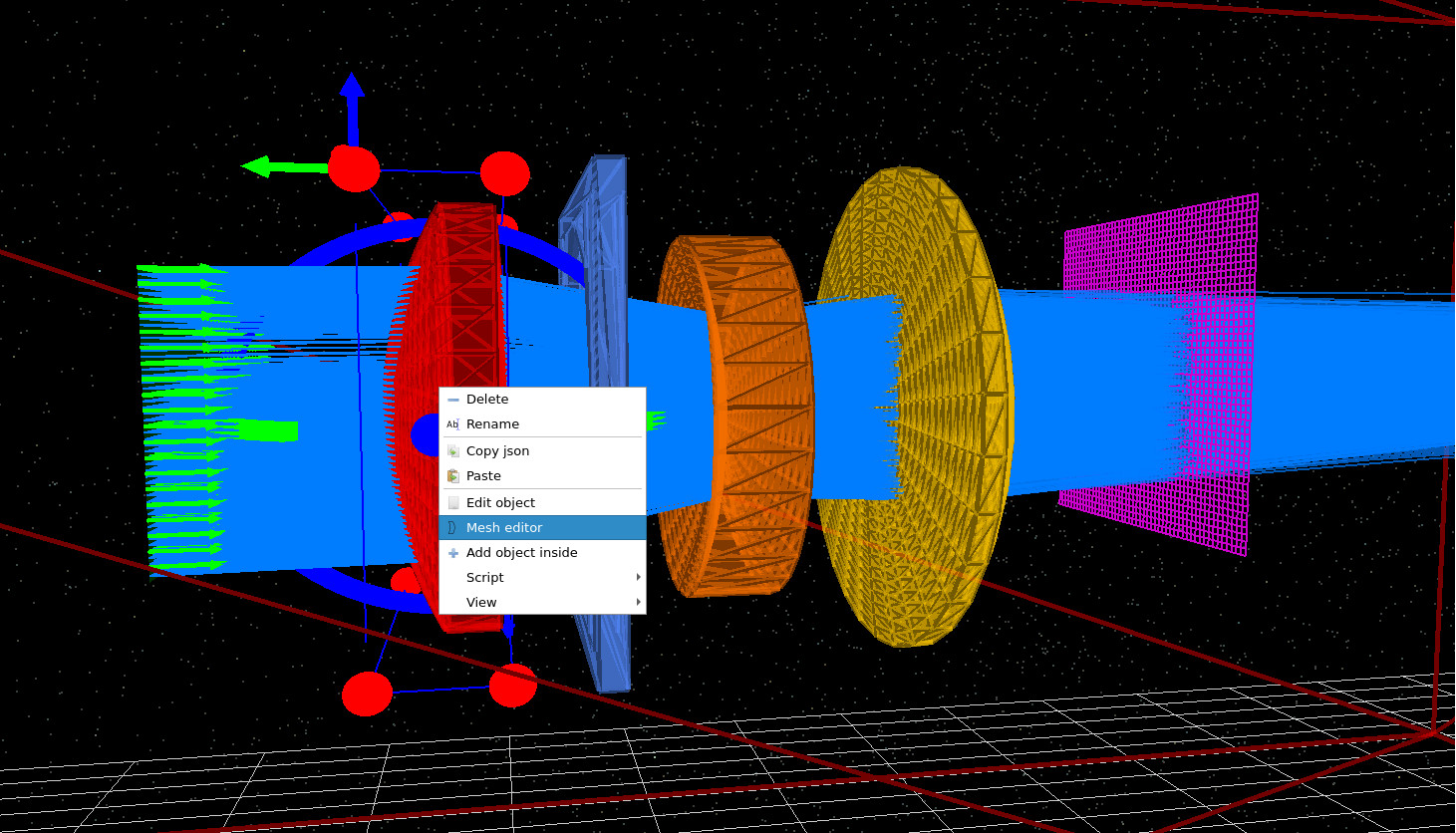
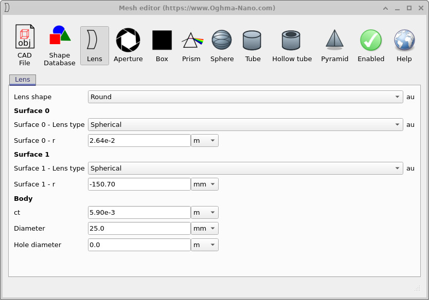
In this step, the geometry of the optical system is modified directly by editing the mesh parameters of the first lens element. To do this, right-click on the first element of the Cooke triplet in the 3D view and select Mesh editor (??). This opens the mesh editor for the selected object, where the physical shape of the lens is defined explicitly in terms of its surface curvatures, thickness, and diameter.
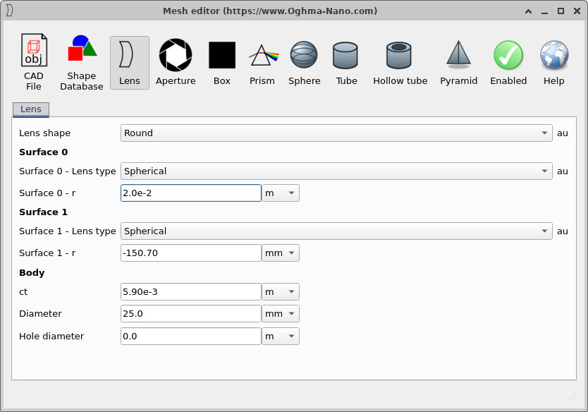
The front surface of the first lens element is labelled Surface 0 in the editor (??). Initially, its radius of curvature is set to 2.64 × 10⁻² m. Reducing this value to 2.0 × 10⁻² m (??) increases the curvature of the surface, making the lens more strongly converging. Although this parameter could also be varied via the S-plane editor, adjusting it directly here is often quicker when exploring the physical effect of individual surfaces.
After updating the curvature, the simulation is re-run (??). Visually, the ray bundle emerging from the first element now converges more strongly, leading to a tighter beam as it propagates through the remainder of the optical system and onto the detector plane. This change in beam shape is subtle in the ray-trace view, but its effect is captured quantitatively in the detector statistics.
The updated figures of merit (??) show a clear reduction in spot size compared to the previous configuration. Both σx and σy decrease, indicating that the beam has become more tightly focused in both transverse directions. The RMS spot radius is correspondingly smaller, confirming that the improvement is not limited to a single axis but reflects an overall sharpening of the image. The encircled-energy radii contract at all energy thresholds, meaning that a larger fraction of the detected power is now concentrated closer to the centroid.
At the same time, the spot ellipticity remains close to unity and the covariance remains small, showing that the increased focusing strength has not introduced significant asymmetry or astigmatism. In physical terms, this simple curvature adjustment improves the convergence of the beam without degrading the overall balance of aberrations in the Cooke triplet. This example illustrates how small, local changes to individual optical surfaces translate directly into measurable improvements in detector-plane performance, and why the figures of merit provide a reliable, quantitative guide when refining an optical design.
6. Summary
In this tutorial, we moved from qualitative inspection of ray traces to quantitative evaluation of optical performance using reproducible figures of merit (FoM). Starting from a Cooke triplet, we showed how detector-plane statistics provide an objective description of image quality that goes beyond visual ray plots.
Using the S-plane and fast optimisation workflow, we generated and ranked design
variants via optimizer_output.csv using metrics such as detector offset,
spot sizes σx/σy, RMS spot radius, spot covariance, ellipse
parameters, encircled energy radii (EE50–EE99), halo energy fraction, encircled-energy
slope, and energy concentration ratios. We also related these numerical metrics to
detector images, RGB composites, and wavelength-resolved snapshots to reveal chromatic
blur, energy concentration, and stray-light behaviour.
Finally, by modifying lens geometry directly and re-evaluating the resulting figures of merit, we demonstrated the core analysis loop: change a physical parameter, re-run the simulation, compare FoM, and validate the result in detector and 3D views. This metric-driven workflow scales naturally from simple lens systems to complex optical designs and provides a robust foundation for optimisation and tolerance-style analysis in OghmaNano.
💡 Next steps: After this FoM tutorial, you may want to explore related optics pages such as Optical detectors, Light sources, or the microlens and optical filtering demo to see how detector configuration, sampling, and system geometry influence the same figures of merit. For an overview of optical systems and ray-tracing simulations, see Optical systems and ray tracing overview.