Cooke Triplet Lens Tutorial (Part A): Optical response
Introduction
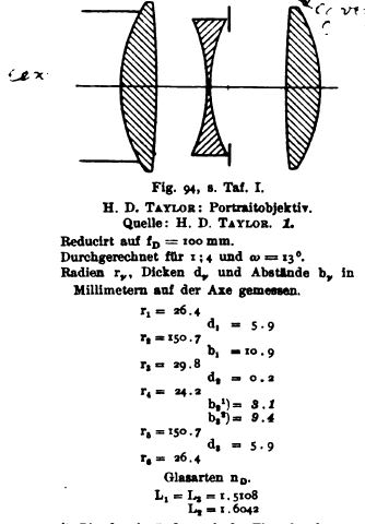
The Cooke Triplet is one of the most influential photographic lenses. Patented in 1893 by H. Dennis Taylor of T. Cooke & Sons, the triplet introduced a new concept in optical engineering: a three-element lens in which a strong positive element at the front and back are separated by a negative meniscus in the centre. This simple but elegant configuration allows the Cooke Triplet to correct a wide range of optical aberrations simultaneously-including spherical aberration, coma, astigmatism, field curvature, and distortion—while remaining compact and manufacturable. For more than a century the Cooke Triplet has served as the basis for many photographic and projection lenses. Modern derivatives of the design continue to appear today in zoom lenses, mobile-phone optics, and compact imaging systems. Its combination of simplicity, tunability, and excellent performance makes it an ideal system for demonstrating optical modelling concepts.
In this tutorial we will use the Cooke Triplet to illustrate the key features of OghmaNano ray tracing tools and S-plane editor, in doing this we will study how the Cooke Triplet affects the optical spectrum of the light that passes through it.
Loading the Cooke Triplet
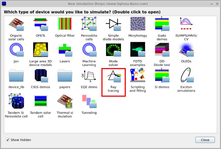
To get started, from the main window click on the New simulation button, this will bring up the new simulation window (??), double-click on the Ray tracing icon. This opens the ray-tracing example library (??).
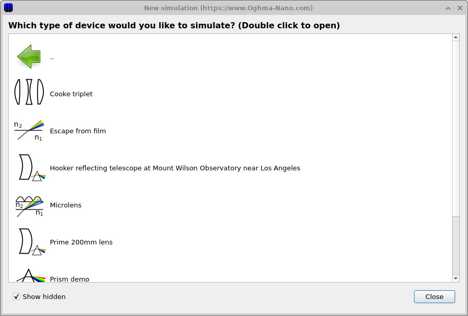
In this list, locate the entry labelled Cooke triplet and double-click it. You will be prompted to choose a directory on your local disk where the simulation files will be stored; select a suitable folder and click OK. OghmaNano opens with the Cooke Triplet scene loaded.
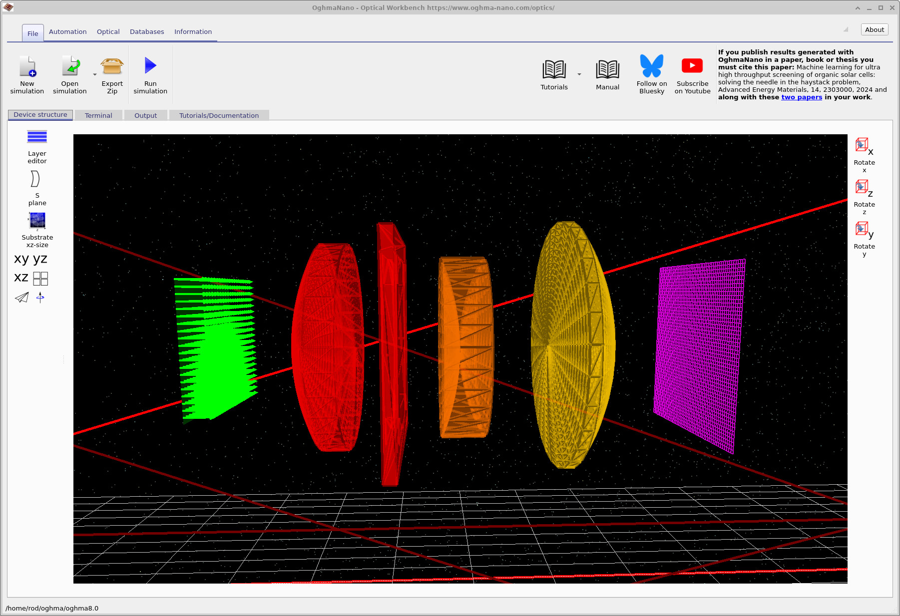
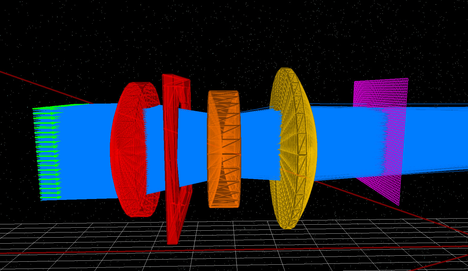
After loading, the main Optical Workbench window will look similar to ??. The three coloured lenses in the centre are the Cooke Triplet elements: a positive (red) front element, a negative (orange) middle element, and a positive (yellow) rear element. On the left is a green plane representing the light source; on the right is a magenta plane representing the image detector. The red flat object is an aperture which controls the amount of light entering the imaging system. In this part of the example it is wide open so all light can pass, and it can therefore be ignored. It is discussed in detail in Part C.
Click and drag with the left mouse button on the black background to rotate the scene. Spend a moment orbiting around the system so you can see how the three lenses and the two planes are arranged in 3D.
Next, open the S-plane editor by clicking the S plane button on the left-hand toolbar of the Device structure tab (also visible in ??). This opens the S-plane table shown in ??.
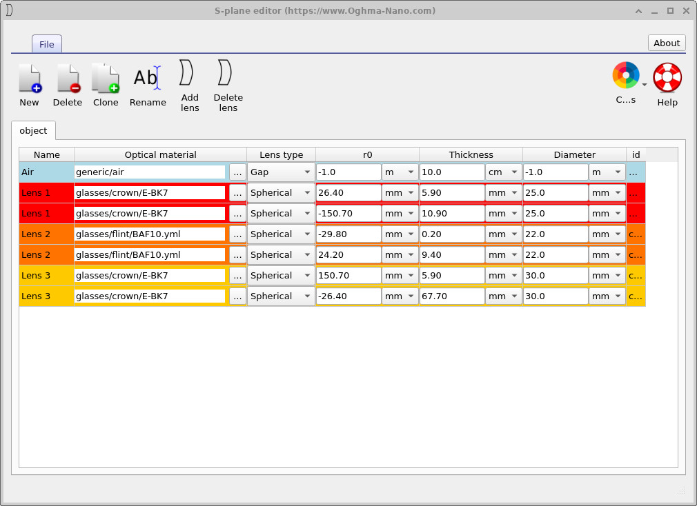
The S-plane editor provides a "surface-by-surface" view of the 3D lens group. Each pair of rows corresponds to the front and rear surfaces of one lens. The columns list the optical material, lens type, radius of curvature r0, thickness, and diameter. Try matching each coloured lens in ?? to its corresponding pair of rows in ??. When you later edit values in this table, the 3D lenses will move and reshape accordingly in the main window.
Although OghmaNano is fully 3D, it is still useful to introduce an S-plane representation, where lenses are decomposed into a sequence of left- and right-hand surfaces. This approach mirrors how many established ray-tracing tools operate, particularly those that are effectively 1D or 2D and assume unidirectional light propagation from left to right through a series of optical surfaces defined by the user. The S-plane view is extremely useful in practice. It allows direct import of surface tables from other optical simulators and from the classical lens-design literature, making it straightforward to reproduce and study historical and modern optical systems. It also provides a compact, intuitive way to edit lens parameters—radii, thicknesses, materials, and apertures—without the overhead of full 3D geometry manipulation.
It should be noted that the S-plane is purely an editing and organisational construct: all rays are still traced in full 3D space, and the resulting optical behaviour is identical to that obtained from an explicit 3D model of the same system.
Running the simulation
Once you are familiar with the geometry, run the ray-tracing simulation by clicking the Run simulation button (blue triangle) in the main toolbar. When the run completes, the scene will look similar to ??, with a blue bundle of rays showing where light has travelled from the source to the detector.
To analyse the results quantitatively, switch to the
Output tab of the Optical Workbench. You will see a list of
files similar to those in
??.
Here, detector0 corresponds to the magenta detector plane.
Double-click detector0 to open its output directory.
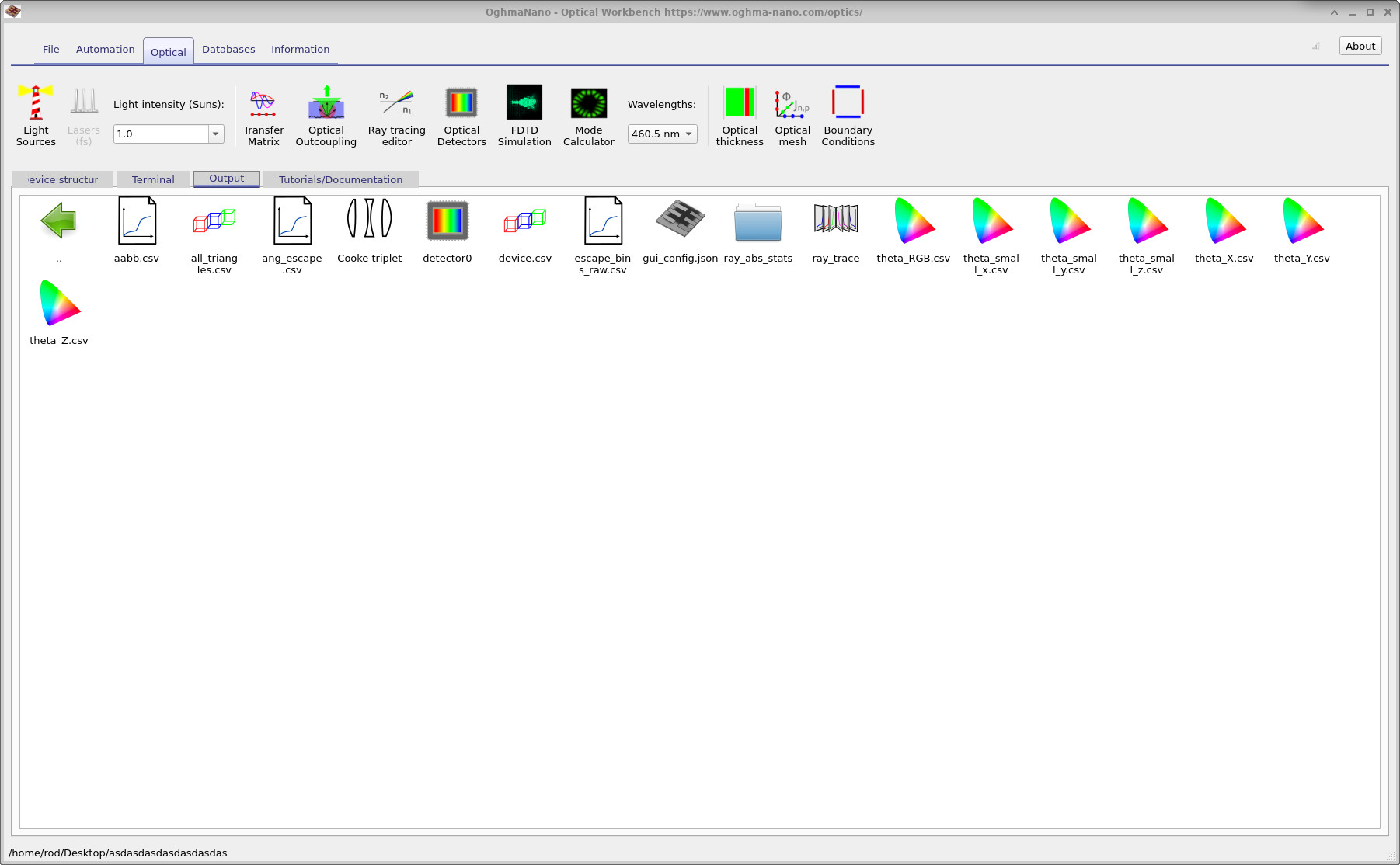
detector0 contains data recorded on the magenta detector plane.
detector0 folder. These include the rendered image and the
wavelength-dependent detection efficiency.
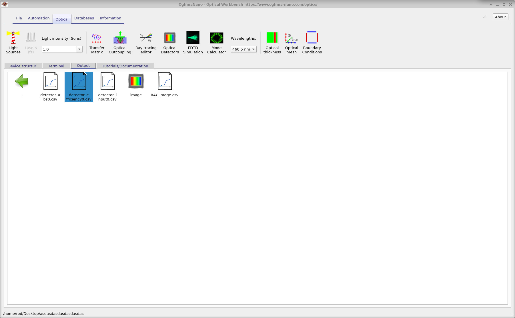
Inside detector0 you will find several result files
(??),
including:
RAY_image.csv– the rendered detector image.detector_efficiency0.csv– overall detection efficiency versus wavelength.
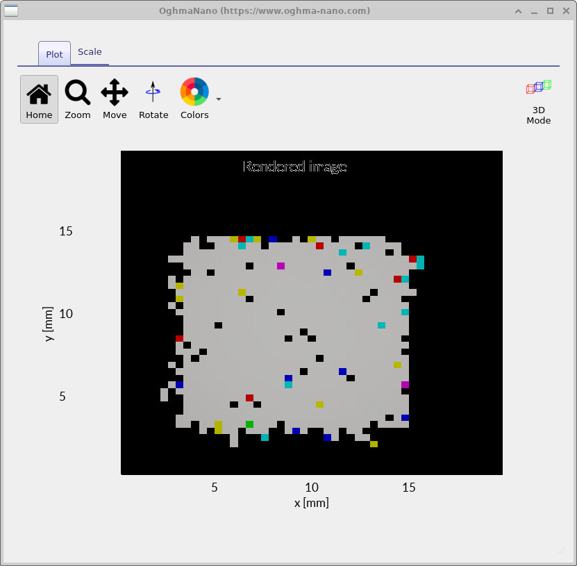
Double-click RAY_image.csv to open the rendered image viewer
(??).
This shows the intensity distribution at the detector plane after passing
through the Cooke Triplet. The image is not perfectly white—the grey tone
reflects the fact that only a fraction of the emitted rays actually reach
the detector, due to reflection and clipping losses within the lens system.
The plot shown in ?? illustrates the wavelength-dependent detection efficiency of the Cooke Triplet. This curve shows the fraction of rays emitted from the source plane that successfully reach the detector after passing through all three lenses. Because each surface introduces reflection, refraction, and potential clipping losses, the collected power is always lower than the emitted power. The gradual increase in efficiency with wavelength indicates that the triplet transmits longer-wavelength light slightly more effectively, a behaviour consistent with reduced refractive-index contrast and lower chromatic deviation at higher wavelengths. This metric is a key indicator of how well the optical system forms an image and how much light is lost internally.

detector_efficiency0.csv. This indicates what fraction of rays from the
source are collected by the detector at each wavelength.
Together, the rendered image and the efficiency-vs-wavelength plot provide a first quantitative look at how well the Cooke Triplet delivers light to the detector. In later sections of this tutorial we will modify lens curvatures and spacings in the S-plane editor and observe how these diagnostics respond.
The effect of the optical system on the light.
In this section we will move the detector plane so that it sits in front of the Cooke Triplet rather than behind it. This helps to separate losses caused by the optical system from those caused by the source or detector setup.
In the main 3D view, click on the detector plane (the purple square). Then, while holding down the Shift key, drag the detector to the left so that it sits just after the light source, as shown in ??. Holding Shift disables object snapping so that you can slide the detector through other objects without accidentally reselecting them.

After repositioning the detector, click the Run simulation button again. Once the ray-trace has
finished, return to the Output tab, open detector0, and then open
detector1. As before, double-click on RAY_IMAGE.csv and
detector_efficiency0.csv to view the new detector image and efficiency plot
(?? and
??).
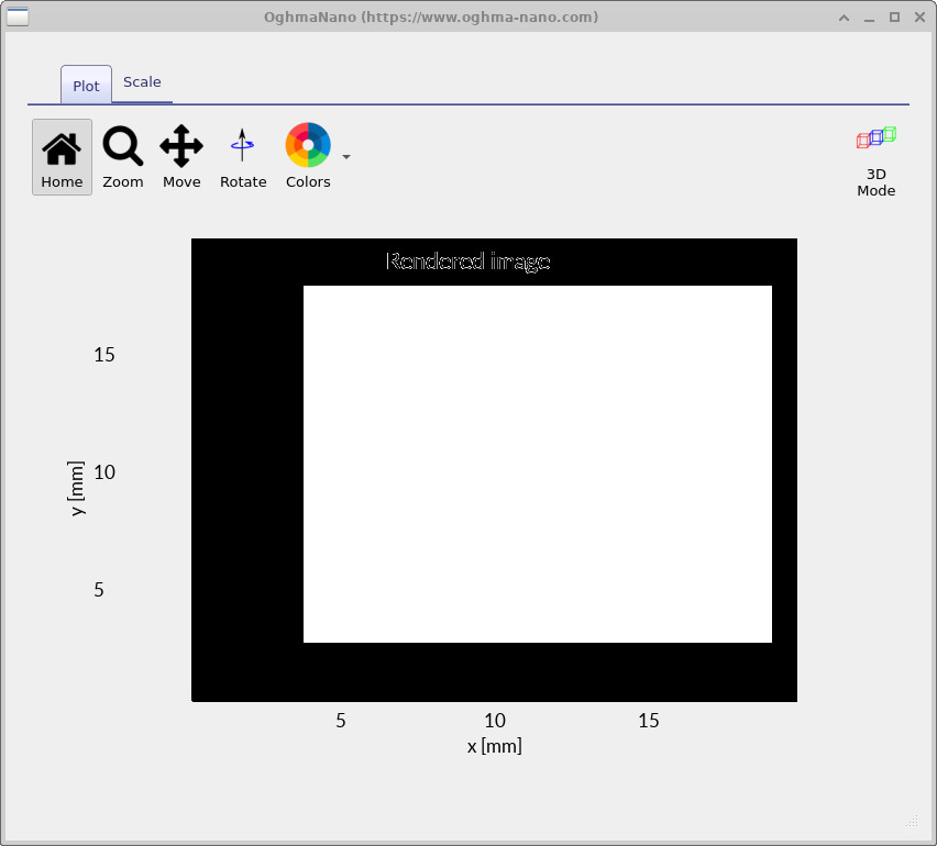

With the detector positioned before the optical system, all emitted rays hit the detector without passing through any glass. As a result, the rendered image is brilliant white and the efficiency curve in ?? is flat at approximately 100 %. For the next step, move the detector back to its original position behind the lens stack so that we can once again analyse the performance of the full Cooke Triplet.
Increasing the wavelength resolution
Up to this point, the Cooke Triplet simulations have been performed using only three wavelengths: red, green, and blue. This is a common approach in colour ray tracing, because three samples aligned roughly with the RGB primaries are sufficient to reproduce colour appearance in rendered images. These three wavelengths correspond to the points shown in ??.
However, while three wavelengths are ideal for colour representation, they are not sufficient for producing accurate spectral plots such as transmission or efficiency curves. To generate wavelength-dependent graphs with meaningful resolution, we need to increase the number of sampled wavelengths.
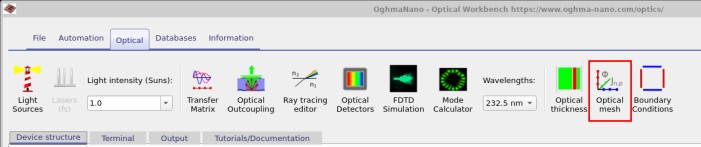
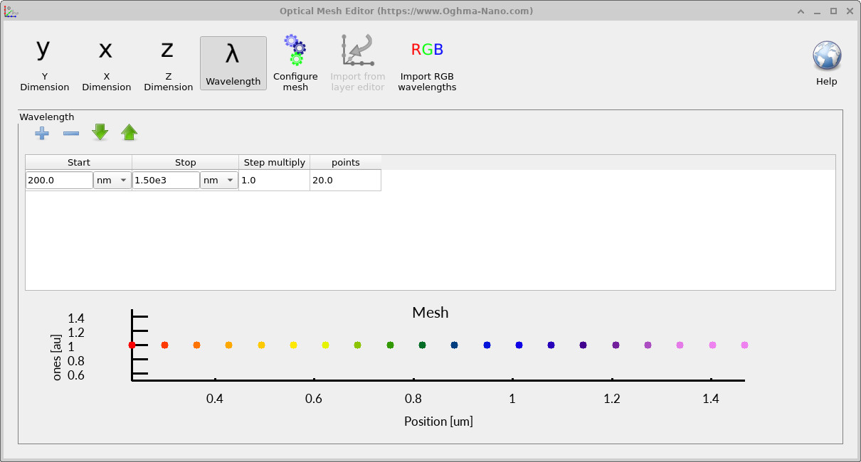
We begin by opening the Optical mesh editor. Go to the Optical ribbon (shown in ??) and click on the Optical mesh button. This opens the current wavelength mesh, shown in ??.
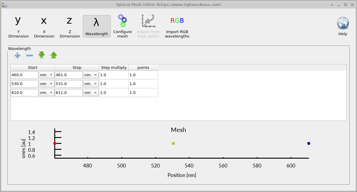
Delete the three existing rows, then click the + button to add a new row. Configure it so that the window matches ??:
- Start: 200 nm
- Stop: 1500 nm
- Points: 20
- Step multiply: 1.0 (uniform spacing)
This gives a much smoother spectral sampling while keeping the computation time manageable. Note that although adding more wavelengths increases simulation time, OghmaNano parallelises wavelength computations across CPU cores. Therefore, on multi-core machines, doubling the wavelength count does not double the wall-clock time.
Now press the Run simulation button again.
Once the simulation completes, return to detector0 and open
detector_efficiency0.csv.
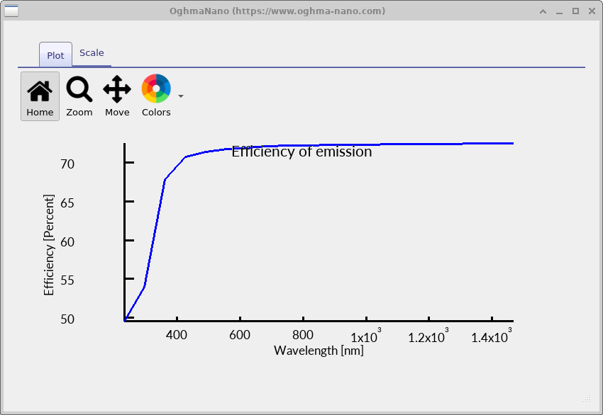
You should now see a smooth spectral efficiency curve, as shown in
??.
The steep decline in efficiency below approximately 300 nm reflects the well-known fact that common optical glasses absorb strongly in the ultraviolet. This physical effect appears in many historical anecdotes. For example, Richard Feynman described observing the first nuclear test from inside a jeep without eye damage because the glass windscreen blocked the harmful UV flash (see his book Surely You're Joking, Mr. Feynman!).
What you can now do (Part A)
- Load and navigate the Cooke Triplet demo in the Optical Workbench.
- Run a ray trace and find the key outputs in
detector0. - Interpret results: read
RAY_image.csvas the detector intensity map, anddetector_efficiency0.csvas the wavelength-dependent throughput of the full lens stack.
Core idea: the detector image tells you where light lands; the efficiency curve tells you how much light makes it through the optics as a function of wavelength.
Common checks if your result looks “wrong”
- Make sure the detector is behind the lens group (not left in front after the diagnostic step).
- Open
detector0(the magenta plane), not a different detector folder. - Keep the wavelength mesh coarse (RGB) for images, and dense (multi-point) for smooth spectra.
👉 Next steps: Now continue to Part B. For an overview of optical systems and ray-tracing simulations, see Optical systems and ray tracing overview.