Cooke Triplet Tutorial (Part C): Aperture Stop, Field Angle, and the Quality–Throughput Trade-off
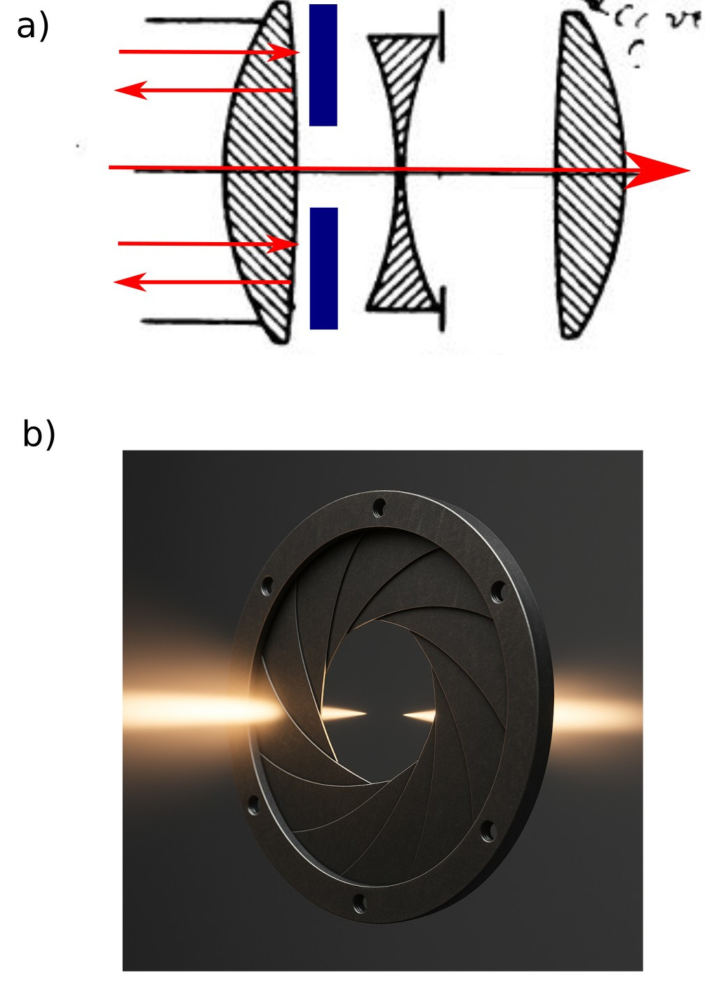
(a) Schematic ray diagram adapted from the original Cooke Triplet lens design by H. D. Taylor (1893), showing the aperture stop placed just behind the first positive element to limit marginal rays. (b) Photorealistic 3D rendering of a mechanical iris diaphragm, illustrating a practical realisation of the aperture stop with light entering and exiting the system.
1. Introduction
The Cooke Triplet is the classic three-element lens form: positive-negative-positive (see Fig. ??a). Historically it became popular because it delivers surprisingly good correction with only three elements, especially for monochrome (or narrowband) imaging, and it forms the "skeleton" that many later photographic objectives build on.
In a real lens, image quality is controlled not only by the glass and surface curvatures, but also by which light rays are allowed to pass through the system. The aperture stop is a physical opening inside the lens (Fig. ??b). Changing its size changes how much of the light beam is allowed through the optics. Making the aperture smaller is called stopping down, while making it larger is called opening up.
When the aperture is wide open, rays from both the centre and the edge of the lens contribute to the image, giving high brightness but stronger optical aberrations (systematic blur). When the aperture is stopped down, many edge rays — called marginal rays — are blocked. This usually improves image quality, but reduces throughput (brightness) because fewer rays reach the detector.
In this tutorial we will build a clean story in two steps: (i) compare wide open vs stopped down for an on-axis beam, then (ii) repeat the same comparison for a slightly tilted beam (field angle). The field-angle case is where the "why" becomes obvious: stopping down usually cleans up off-axis aberrations such as coma/astigmatism, but you pay in light.
2. Make the light source slightly larger
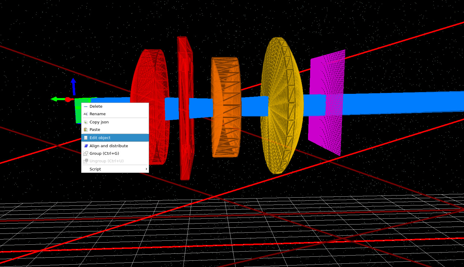
Begin from your working Cooke Triplet scene. In the 3D view, right click on the light source and select Edit object, as in ??. This opens the light/object editor where we will slightly increase the source footprint. Keep everything else fixed (same lenses, same detector position, same wavelength mesh). This small change will just make the diagrams we produce later easier to interpret.
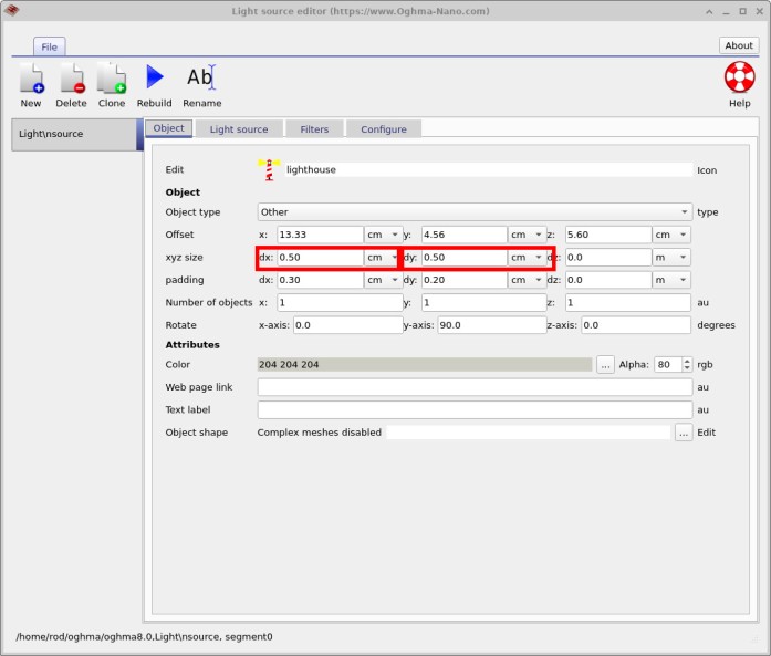
dx = 0.5 cm and dy = 0.5 cm. This makes the demo slightly easier without changing the underlying optics.
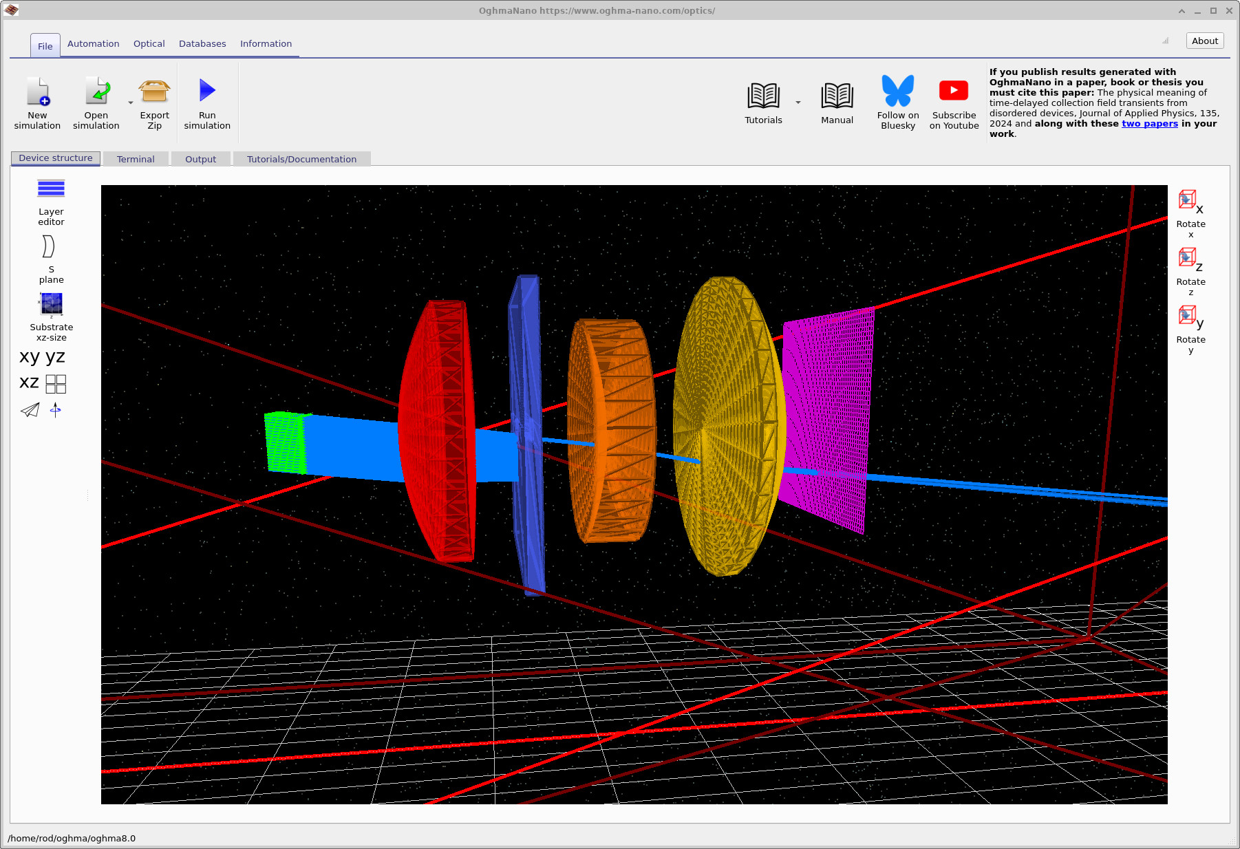
3. On-axis baseline - wide open vs stopped down
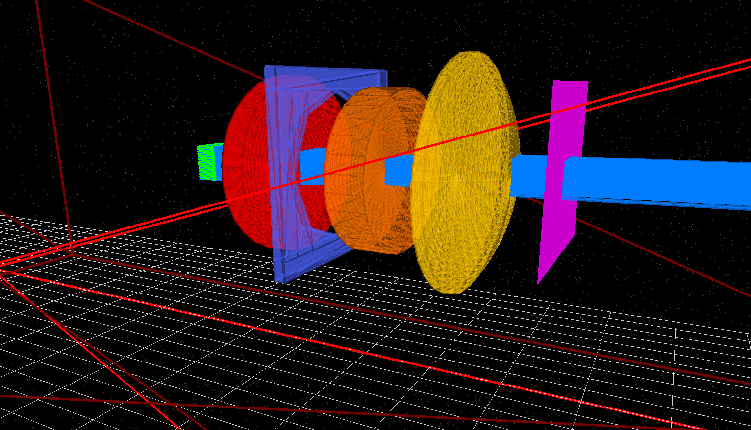
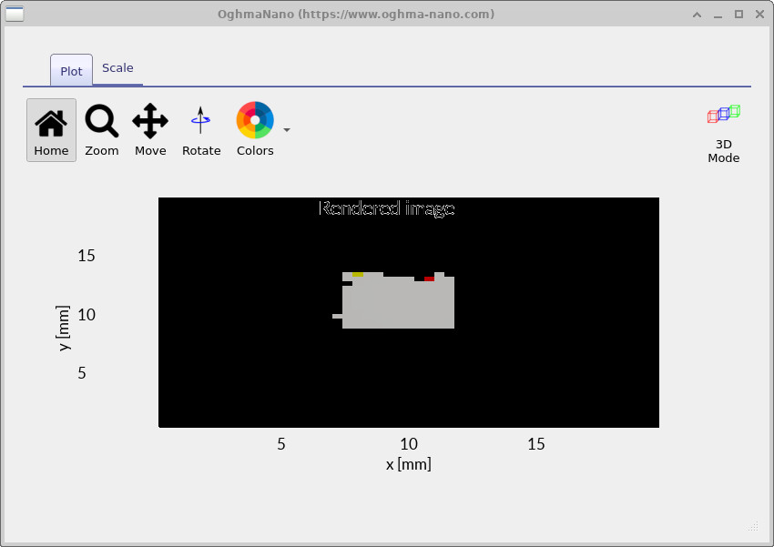
First we establish an on-axis reference case. Run the simulation with the aperture wide open. Rotate the 3D view so it matches ??. You should see the aperture clearly as a blue circular opening in a square plate. In this configuration the opening is large, so the beam passes cleanly through the first lens, the aperture, the second lens, and the third lens, and then reaches the detector without being clipped.
Run the simulation and open the detector output. Load the file
RAY_image.csv; this image is your before case and will be used
as a reference throughout the rest of this tutorial.
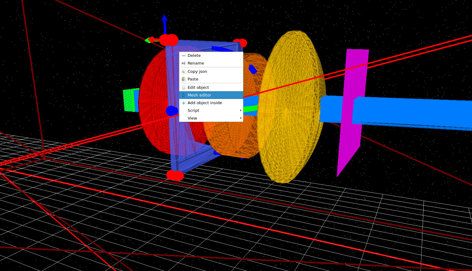
Next, we will stop down the aperture, meaning we deliberately make the
opening smaller so that some rays are blocked. Right click the aperture and select
Mesh editor
(??),
then set the aperture diameter parameter
D0 to 0.002 m
(??).
Re-run the simulation. You should now see strong clipping in the 3D view: many rays
terminate at the aperture, and only a reduced subset reaches the detector.
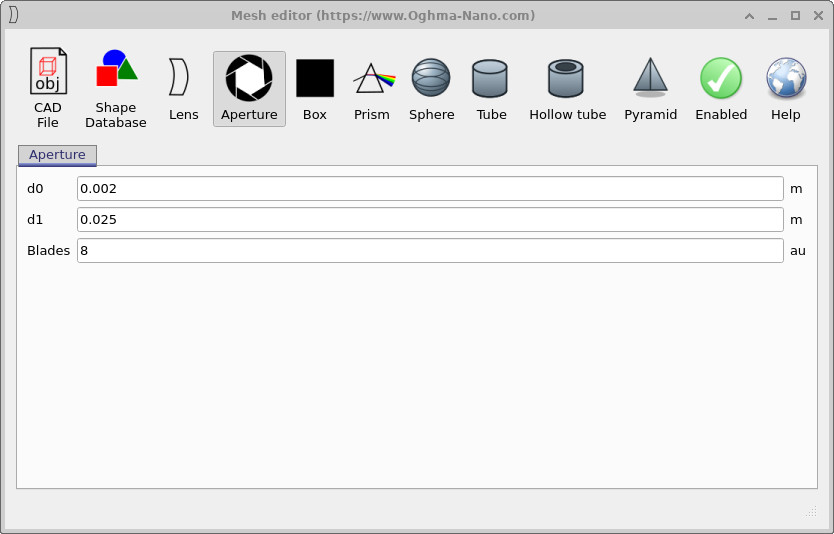
D0 = 0.002 m.
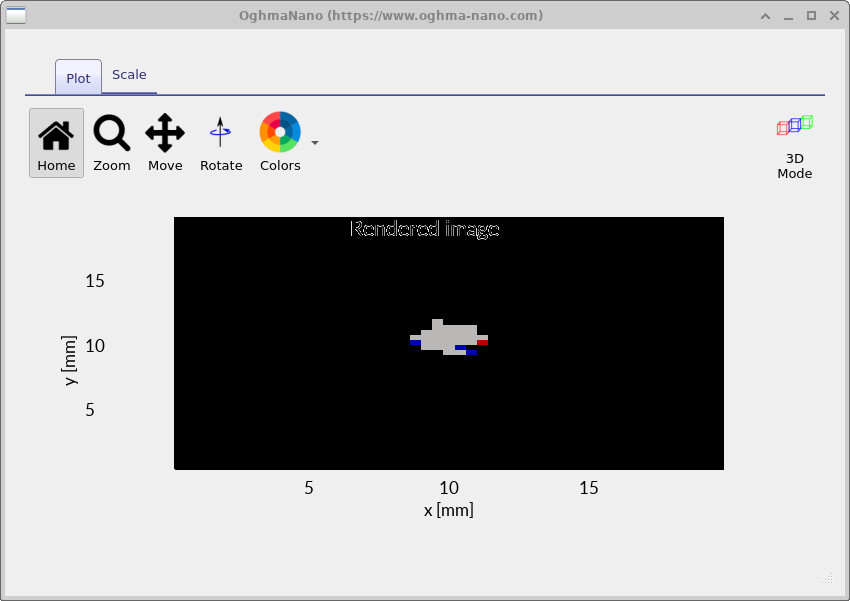
Open RAY_image.csv in detector 0. Compared to the wide-open case, the
spot is now noticeably smaller and cleaner. This is because stopping down removes
marginal rays, meaning rays that travel through the outer edges of the lens,
which are the most strongly affected by spherical aberration in a simple three-element
system like the Cooke Triplet. The remaining paraxial rays (rays close to the
optical axis) focus more nearly to the same point, improving image sharpness at the
expense of optical throughput (the total amount of light reaching the detector). In
practical terms, the lens produces a dimmer but better-corrected on-axis image, which
is the fundamental trade-off controlled by the aperture stop.
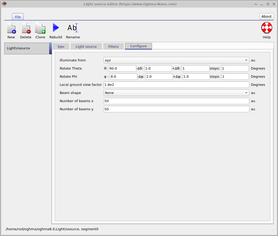
4. Introduce field angle by pointing the beam slightly down (Rotate Phi)
Now we repeat the same open/closed comparison, but with a small field angle. In classical optics, an off-axis object at infinity is represented by a bundle of rays that are still (approximately) parallel to each other, but tilted relative to the optical axis. In OghmaNano, you can do this directly in the light source editor.
Open the light source editor again and go to the Configure tab. Find the line
Rotate Phi and set phi = 8 degrees, as in
??.
This “points” the beam slightly downward through the lens, mimicking light coming from a point
that is not exactly on the optical axis (i.e. not at the centre of the field of view).
In real imaging systems most objects are off-axis, especially toward the edges of an image.
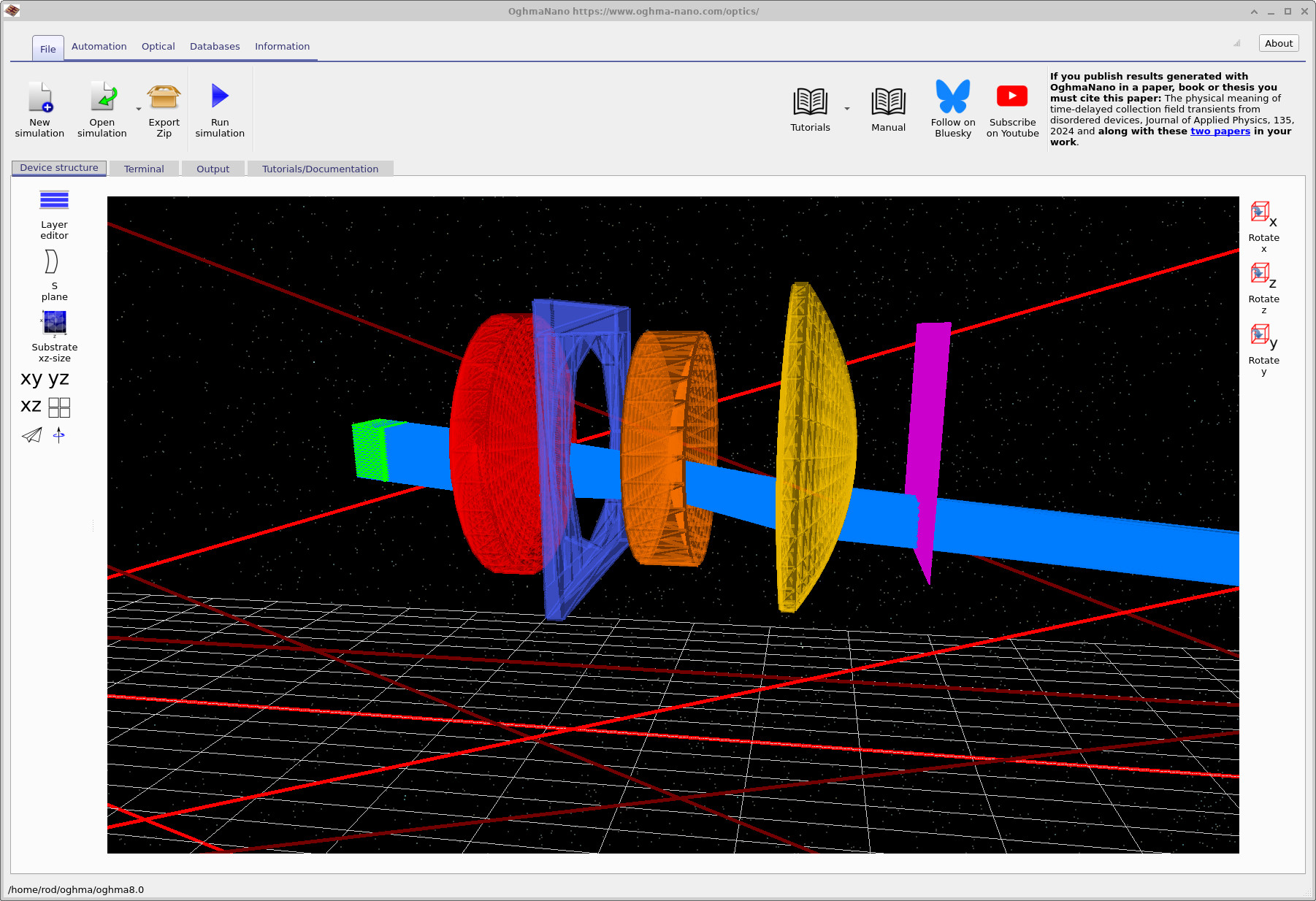
With phi = 8°, run the simulation with the aperture still stopped down
(small D0). You should see that most rays are rejected at the aperture, and only a
narrow subset continues through the lens stack to the detector
(example in ??).
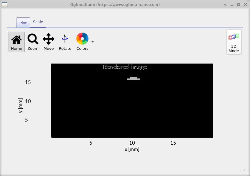
If you open the detector image you should see a small, compact spot
(example in ??).
A small spot on the detector means that light from a single point in the scene is brought to nearly the same location in the image. This corresponds to sharper detail and higher resolution, because neighbouring points in the object are less likely to blur together. In practice, a lens that produces small spots can form clearer, more accurate images, even though it may be dimmer when the aperture is stopped down.
phi = 8°) with the stop closed: most rays are absorbed at the aperture; only a small fraction makes it through.
5. Field-angle comparison — stopped down vs wide open
Now open the aperture again (set the stop back to wide open) and re-run the simulation with the same field angle. With the aperture open, many more rays are allowed through the lens, including rays that pass through the outer regions of the optics. These marginal rays do not focus to the same point as the central (paraxial) rays, especially for off-axis light. As a result, the detector image typically shows a larger footprint and increased distortion: light from a single off-axis point is spread over a wider area rather than forming a compact spot. This comparison highlights why lenses often perform poorly at the edges of the field when used wide open, and why stopping down is an effective way to control off-axis aberrations, at the cost of reduced brightness.
phi = 8°) with the stop opened up: many more rays pass through the lens system and reach the detector.
🧪 Exercise — Aperture sweep at fixed field angle
Keep the field angle fixed at phi = 8° and run a series of simulations while sweeping
the aperture size (choose several values of D0, from wide open to strongly stopped
down). For each run, record a simple image metric such as spot size, centroid shift, or total
detector counts.
Plot your chosen metric versus D0. The resulting curve is a genuinely useful optical
result: it directly shows how image quality and throughput trade off with f-number, which is
exactly the kind of data used to compare and tune real lens designs.
🔍 What should you expect to see?
As D0 is reduced (the aperture is stopped down), image quality metrics such as
spot size should generally improve, especially for this off-axis case. This happens because
highly aberrated marginal rays are progressively removed, leaving mostly near-paraxial rays
that focus more consistently.
At the same time, the total detector counts will fall rapidly, because fewer rays are admitted into the system. The resulting curves typically show a clear trade-off: strong improvement in image quality at first, followed by diminishing returns as the aperture becomes very small.
In a more advanced model you would eventually see diffraction limit the spot size at very small apertures, but in this geometric ray-tracing tutorial the dominant effect is aberration suppression versus throughput loss.
Conclusion and next steps
You now have a clear, reproducible demonstration of one of the central trade-offs in lens design: using a lens wide open maximises brightness, while stopping down improves image quality, most noticeably for off-axis light. By introducing a controlled field angle using Rotate Phi, you have also established a systematic way to explore how classical aberrations such as coma, astigmatism, field curvature, and lateral colour emerge in real optical systems.
👉 Next steps: For an overview of optical systems and ray-tracing simulations, see Optical systems and ray tracing overview.