Ray-Tracing Tutorial (Part A): Prism and Teapot Playground

🎯 Learning objectives

Load and run a basic 3D ray-tracing simulation in OghmaNano.
Identify sources, prisms, apertures and detectors in the ray-tracing view.
Visualise reflection, refraction and dispersion in a prism system.
Inspect detector outputs (efficiency curves and rendered images).

📦 Prerequisites

OghmaNano installed and working.
Basic familiarity with Snell’s law and reflection/transmission.

⏱ Estimated time

Part A: 10–15 min
Later parts (B, C…): 15–20 min each
In total around 1 hr depending on how much you explore.

📺 YouTube examples

Running a simple ray-tracing simulation in OghmaNano.

In this tutorial you will use OghmaNano’s Optical Workbench to play with a colourful ray-tracing scene containing prisms, an aperture, a detector and (in later parts) a CAD teapot. The aim is not to build a realistic camera, but to give you a playground for exploring the main features: launching simulations, rotating objects, looking at beam profiles and examining what the detector “sees”.

We start from a pre-built prism demo. This scene already includes:

Two red prisms in the optical path.
A green ray source that launches photons into the system.
An aperture that blocks rays away from the central hole.
A purple detector that collects all rays that pass through it.

When you run the simulation you will see reflection, refraction and dispersion in action, and you will be able to inspect both the detector efficiency and a rendered image of what the detector views.

Step 1: Create a new ray-tracing simulation

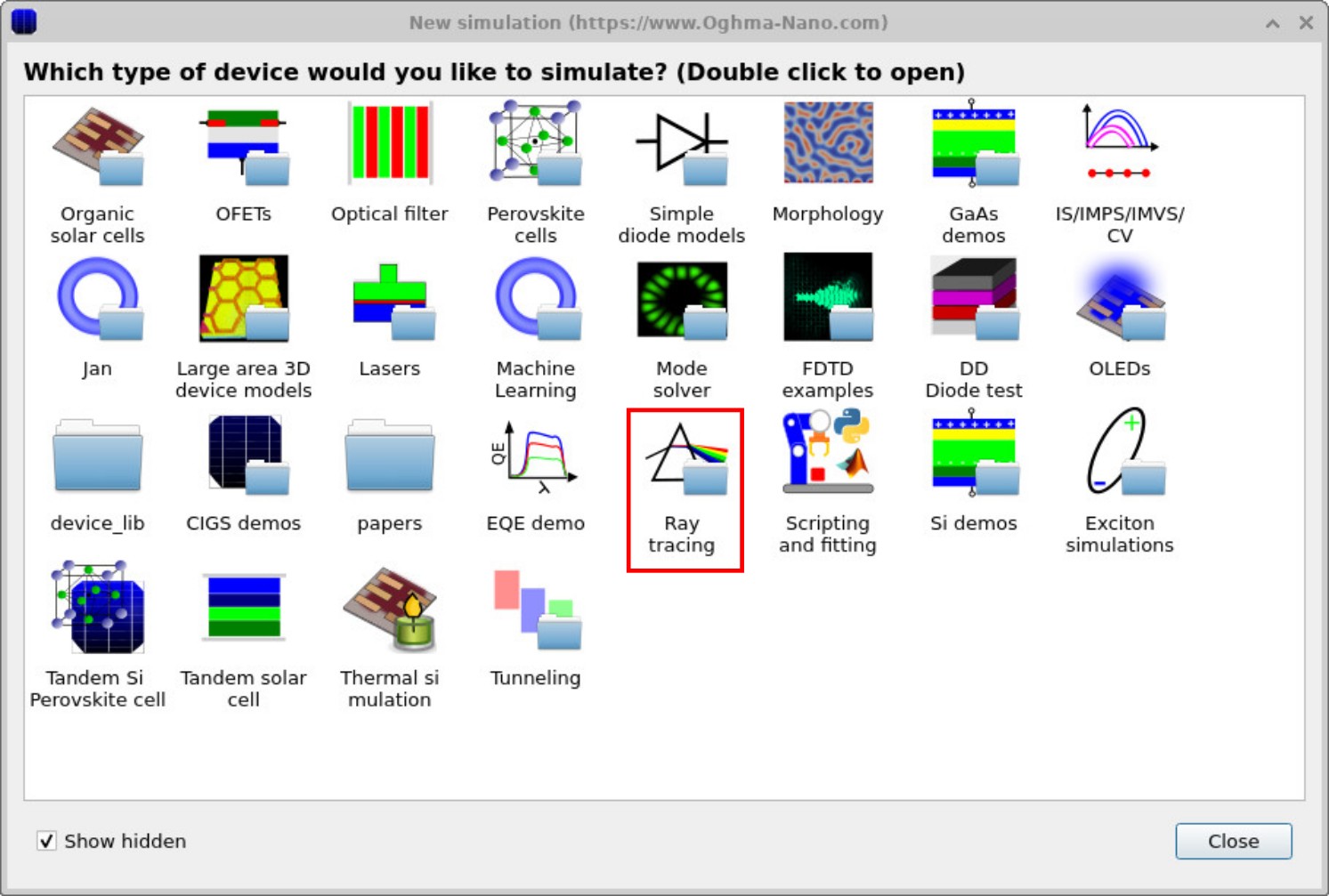
Start OghmaNano from the Windows Start menu. From the start window select New simulation. This opens the device-library window shown in ??. Double-click the Ray tracing folder (highlighted) to open the list of ray-tracing examples, shown in ??.

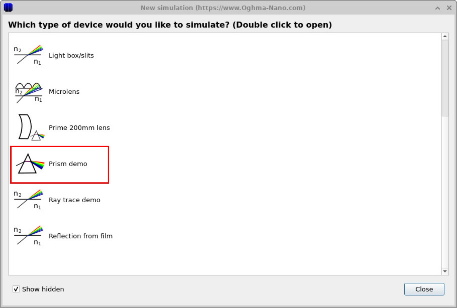
OghmaNano new simulation window with the Ray tracing examples folder highlighted — The *New simulation* window. Select the **Ray tracing** folder to open the ray-tracing examples library.

Ray-tracing examples window with the Prism demo highlighted — Inside the **Ray tracing** library select the **Prism demo**. This example contains two prisms, a source, an aperture and a detector.

Double-click Prism demo, then choose a folder where you have write access and save the simulation. For best performance save to a local disk (for example C:\) rather than a network or cloud drive.

Step 2: Explore the default scene

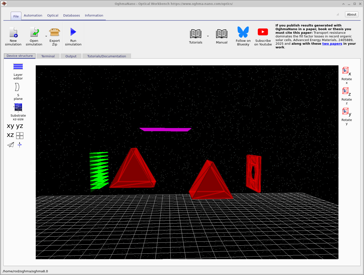
After loading the example, the main Optical Workbench window opens as shown in ??. The scene contains the main optical components you will use throughout this tutorial:

Green arrows (left): an optical source that launches rays of different wavelengths.
Two red prisms: bulk optical elements that refract and reflect the rays.
Red aperture plate: a plate with a central opening that lets some rays through while blocking others.
Purple grid (top): a detector that collects rays, similar to a CCD in a camera.

Use the mouse to look around the scene. The left mouse button rotates the view, while the right mouse button pans the scene. You can zoom in and out using the mouse wheel. On the left-hand side of the window you will see buttons labelled XY, YZ, and XZ. These preset the camera to look directly along each plane, which can be useful when repositioning objects or checking alignment.

Optical Workbench simulation window showing prisms, a detector, a source and an aperture — The default **prism demo** scene. Two prisms sit between the green source and the purple detector. A red aperture plate on the right allows only rays passing through its central opening to continue.

Ray-tracing simulation running, showing coloured rays reflecting and refracting through the prisms and aperture — After running the simulation, coloured rays propagate from the source, refract inside the prisms, and either pass through or are blocked by the aperture before reaching the detector.

Step 3: Run the simulation

Click the Run simulation button (blue play icon) or press F9. OghmaNano traces rays from the source, through the prisms and aperture, to the detector. When the run finishes the scene looks similar to ??.

The coloured bands show how different wavelengths follow different paths through the prisms. This is a simple demonstration of:

Snell’s law (refraction at an interface),
Reflection at boundaries, and
Dispersion – different refractive indices for different wavelengths, leading to a visible rainbow. (See the Wikipedia article on optical dispersion for background.)

Snell’s law and reflection/transmission

Snell’s law relates the angles of incidence and refraction at a flat interface:

\( n_1 \sin\theta_1 = n_2 \sin\theta_2 \)

where \(n_1\) and \(n_2\) are the refractive indices of medium 1 and 2, and \(\theta_1\) and \(\theta_2\) are the angles measured from the surface normal.

At normal incidence a simple expression for the power reflectance \(R\) at an interface is

\( R = \left(\dfrac{n_1 - n_2}{n_1 + n_2}\right)^2 , \qquad T = 1 - R \)

where \(T\) is the transmitted fraction of power. OghmaNano uses these ideas (together with the full Fresnel equations) when tracing each ray through the prisms and aperture.

Step 4: Inspect the detector outputs

To see what the detector has recorded, click the Output tab at the top of the window. You will see the list of files written by the ray tracer, similar to ??. The most important file at this point is the detector0 folder, which stores the outputs from the purple detector.

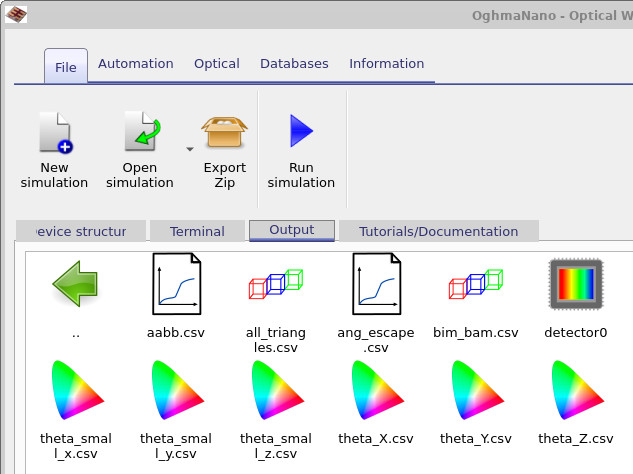
Output tab showing the detector0 folder and other ray-tracing result files — The **Output** tab for the prism demo. The `detector0` icon contains all results associated with the main detector: efficiency curves, images and CSV data.

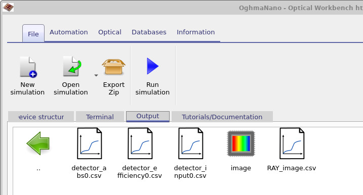
Contents of detector0 showing detector_abs0.csv, detector_efficiency0.csv, detector_input0.csv and RAY_image.csv — Inside `detector0` you will find the main detector output files, including `detector_efficiency0.csv` (efficiency vs wavelength) and `image` (a rendered view of the detector field).

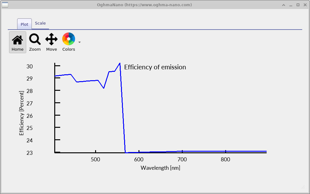
Double-click detector0. Then double-click detector_efficiency0.csv to plot how efficiently the detector collects light as a function of wavelength, as shown in ??.

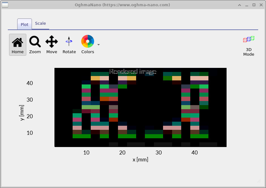
Detector efficiency plot showing efficiency of emission versus wavelength — The detector efficiency spectrum. In this example around 23–29 % of the rays at a given wavelength reach the detector, depending on how they are refracted and blocked by the prisms and aperture.

The RAY_image.csv file shows a rendered picture of what your eye would see if it were placed in the detector plane. Note the “hole” in the centre of the beam where the aperture has blocked rays.

Next, double-click the RAY_image.csv file. OghmaNano reconstructs a colour image from all the wavelengths that reached the detector (typically around 20 wavelength bins in this demo). Rays that went through the central opening in the aperture form the bright coloured region on the detector; rays blocked by the aperture leave a dark hole in the beam profile.

If you rotate the 3D scene and follow the rays visually, you can trace how this hole forms: some rays are reflected by the aperture plate, some miss the detector entirely, and only rays that pass through the opening contribute to the bright region in ??.

👉 Next step: Continue to Part B from prisms to lenses.