Ray-Tracing Tutorial (Part E): Materials and the World Box

In this final part we will finish the simple ray-tracing playground by changing the optical material of the teapot and then displaying the world box that defines the simulation limits. By the end, you should be comfortable editing both geometry and materials, and know how far you can move objects before they fall outside the simulated world.

Step 1: Change the teapot material

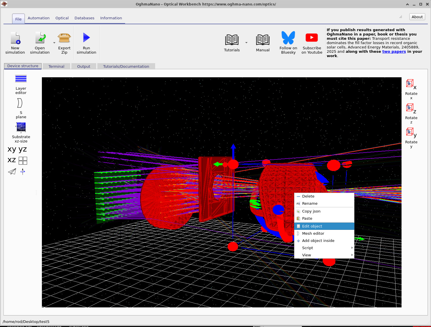
Start from the scene created in Part D, where the teapot has already been imported from the shape database and placed in the beam. Right-click directly on the teapot mesh and choose Edit object from the context menu. This opens the general Object editor, shown in ??.

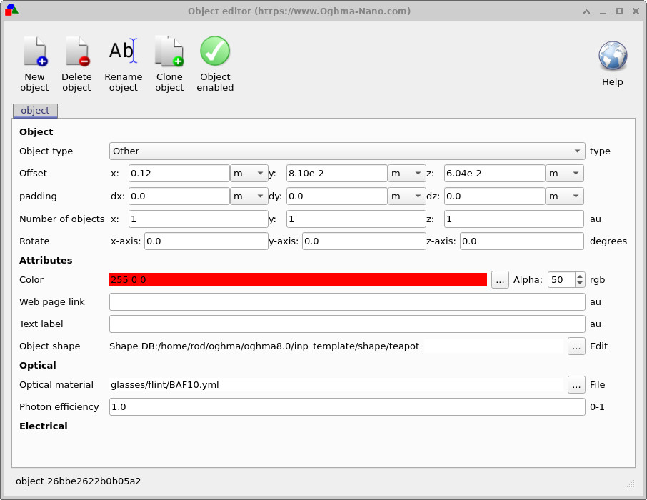
In the Object tab of the editor you can see the teapot position, rotation and colour. For this step we only need the Optical section at the bottom:

1. Locate the field Optical material.
2. Click the ... button next to it.
3. In the file chooser that opens, select the material glasses/flint/BAF10.yml.
4. Click Open to confirm, then close the object editor window.

The teapot now uses the high-index flint glass BAF10 from the optical database. When you re-run the simulation, rays will refract more strongly as they enter and leave the teapot compared to a lower-index material.

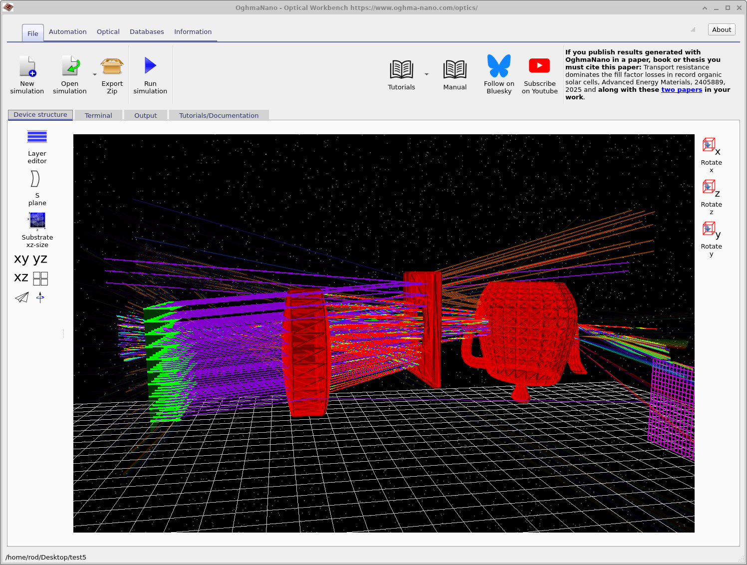
Click Run simulation (or press F9). After the ray trace finishes, you should see something similar to ??, with rays entering the teapot, refracting inside, and emerging on the far side.

Step 2: Display the world box

Every object in the scene lives inside a finite world box. This box defines the region within which the ray tracer expects to find objects. Rays interacting with shapes far outside the box may be ignored or cause the simulation to complain about invalid geometry.

To visualise the world box:

1. Right-click anywhere in empty space (not on an object) in the Optical Workbench view.
2. From the context menu choose View > Optical > Show world box, as shown in ??.

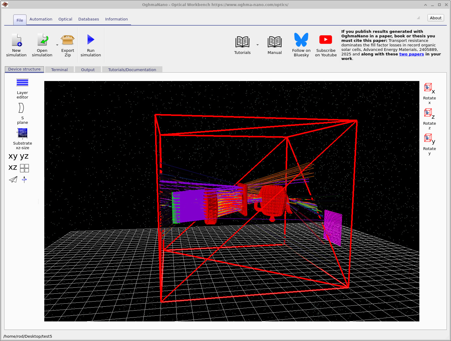
Once enabled, the world box appears as a large red wireframe cube (or rectangular box) surrounding your optical system, as in ??. You can still move and rotate objects freely, but if you drag them far outside this box:

• they may no longer interact with rays in the way you expect, and
• the solver may warn that the geometry is invalid or outside the simulation domain.

To change the size of the world box, use the control in the left-hand panel labelled Substrate xz-size. This defines the lateral extent of the virtual world in the x–z plane. Increasing it gives you more space to place objects, while decreasing it focuses the simulation on a smaller region around the optical system.