Ray-Tracing Tutorial (Part C): Moving Detectors
In the previous parts you edited prisms and lenses to build up a simple optical system. In this part you will focus on the purple detector. Detectors in OghmaNano are defined as flat planes (a bit like a CCD sensor): whenever a ray hits this plane, it is recorded in the detector output files.
Step 1: Open the detector editor
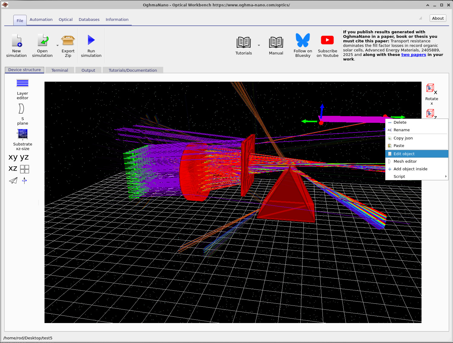
Start from the scene you finished in Part B (lens, prisms, aperture and detector). Locate the purple detector plane. Right-click on it and select Edit object from the context menu, as shown in ??. This opens the general object editor window in ??.
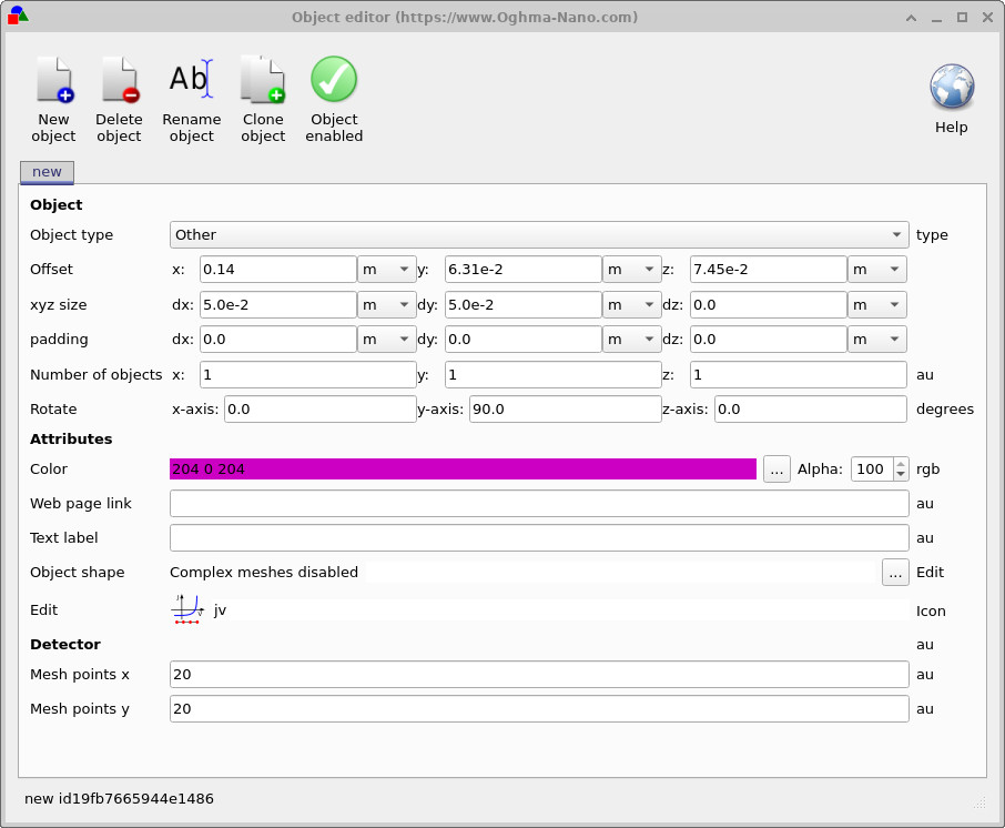
dx, dy), rotation and the number of mesh points (detector pixels).
The detector is defined as a rectangular plane with physical dimensions:
- dx – size in the x direction (width),
- dy – size in the y direction (height).
In ?? the detector is
set to dx = 5.0e-2 m and dy = 5.0e-2 m, i.e. a
5 cm × 5 cm sensor.
At the bottom of the editor you will also see:
- Mesh points x = 20
- Mesh points y = 20
This means the detector is divided into a 20 × 20 grid of bins – effectively 400 coarse “CCD pixels”. This is much lower resolution than a real camera, but it is usually sufficient when tracing rays through optical systems and keeps simulation time reasonable. You can always increase these values later if you need a finer beam profile.
Step 2: Rotate the detector plane
In the object editor you can also see the detector’s orientation. In this example the detector has already been rotated around the y-axis by 90° so that it faces the incoming rays. To understand how rotation works, change the settings as follows:
- Set Rotate x-axis to
90.0degrees. - Set Rotate y-axis to
90.0degrees.
The detector is internally defined as a flat plane in the x–y plane. By rotating it 90° around both the x and y axes you flip it from a near-horizontal orientation to a clearly vertical plane in the scene. Close the editor and check that the detector now appears upright when viewed in the 3D window.
Step 3: Move the detector closer to the aperture
Next, move the detector so that it sits just behind the aperture. This will give you a clearer beam profile and a more compact optical setup.
- In the main Optical Workbench window, left-click directly on the purple detector plane.
- Drag it towards the aperture surface. Make sure your mouse is over the detector itself (not empty space behind it) so that the correct object is selected.
- If the detector collides with the prism or other objects and refuses to move further, hold down Shift while dragging. This temporarily overrides collision detection and lets you move the detector through other meshes.
Position the detector roughly as shown in ??.
Step 4: Tidy the scene (optional)
To simplify the playground you can remove one of the prisms. Right-click on the prism and select Delete. You should now be left with a scene containing:
- One lens,
- One aperture plate,
- One detector plane.
Run the simulation again. With the detector placed close to the aperture the beam profile will be sharper and it becomes easier to see how the lens focuses rays onto the detector area.

👉 Next step: Continue to Part D to learn how to insert new object into the scene.