Poisson Equation and Electrostatics in Drift-Diffusion Models

Electrostatics is a central component of drift-diffusion modelling, determining how electric potential, charge density, and energy levels vary across a device. The electrostatic potential controls band bending, carrier distributions, and ultimately recombination and transport processes.

1. Definition

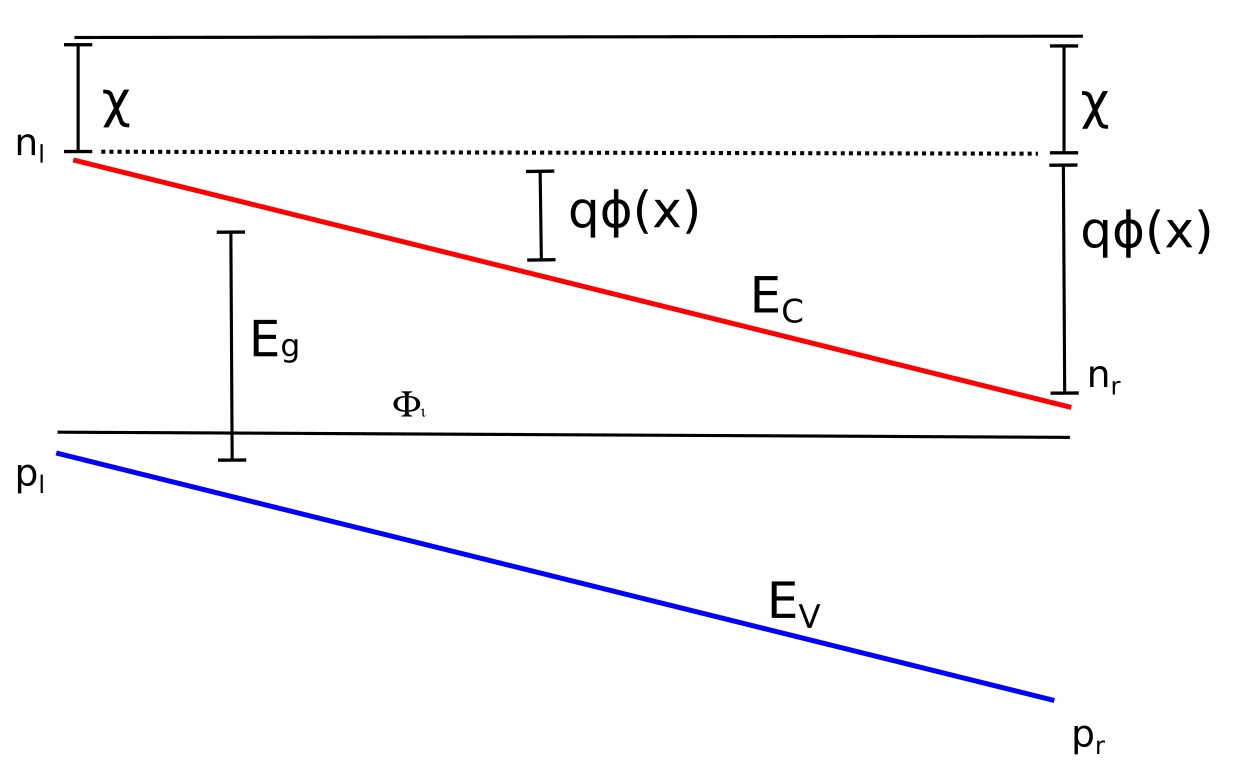
Energy band diagram showing conduction band (Ec) and valence band (Ev) under an internal electric field, with spatially varying electron and hole densities (n_l, n_r, p_l, p_r), bandgap Eg, and electrostatic potential qϕ — Energy band diagram illustrating spatial variation of the conduction band (\(E_C\)) and valence band (\(E_V\)) under an internal electric field. The bandgap \(E_g\), electrostatic potential \(q\phi\), and carrier densities (\(n_l, n_r, p_l, p_r\)) are indicated. This representation highlights how carrier populations and energy levels vary across a device, providing the framework within which free-to-free recombination occurs.

The energy band diagram shown in ?? illustrates how the conduction and valence band edges vary across a device. The red line corresponds to the conduction band edge \(E_C\), while the blue line corresponds to the valence band edge \(E_V\). The separation between them defines the band gap \(E_g\).

To define the absolute energy scale, we introduce the electron affinity \(\chi\), which sets the energy difference between the vacuum level and the conduction band edge in the absence of an electrostatic potential. This provides a material-dependent reference for the band structure.

In the presence of an electrostatic potential \(\phi(x)\) (caused by charge), the conduction band edge is shifted by the electrostatic energy \(-q\phi(x)\), so that

\[E_{\mathrm{C}}(x) = -\chi - q\phi(x)\]

The valence band edge is then obtained by subtracting the band gap \(E_g\),

\[E_{\mathrm{V}}(x) = -\chi - E_g - q\phi(x)\]

The spatial variation of \(E_C(x)\) and \(E_V(x)\), shown in ??, arises from the position dependence of the electrostatic potential \(\phi(x)\) (in the absence of heterojunctions). This potential is obtained self-consistently by solving Poisson’s equation across the device, and directly determines the band bending that governs carrier transport and recombination.

2. Calculating the electrostatic potential from charge

In semiconductor device physics, the electrostatic potential is calculated from Poisson’s equation, which relates the divergence of the electric field to the local charge density:

\[ \nabla \cdot \bigl( \epsilon_0 \epsilon_r \nabla \phi \bigr) = -q \left( n_f + n_t - p_f - p_t - N_{ad} + N_{ion} + a \right), \]

where \(n_f\) and \(p_f\) are the densities of free electrons and holes, while \(n_t\) and \(p_t\) are the corresponding trapped carrier densities. The term \(N_{ad}\) represents the ionized dopant density, \(N_{ion}\) accounts for background ionic charge (for example, fixed ions in perovskite layers), and \(a\) denotes mobile ions that can drift in response to the local field. The permittivities \(\epsilon_0\) and \(\epsilon_r\) set the strength of the electrostatic response.

This formulation captures all relevant contributions to space charge: free and trapped carriers, intentional doping, and both static and mobile ionic species. It is particularly important for hybrid materials such as organics and halide perovskites, where ionic motion and trap states strongly influence the electrostatic potential and give rise to phenomena such as hysteresis and slow transients.

👉 Next step: Now continue to The drift-diffusion equations

👉 Or: See how electrostatics affects real devices in the pn junction tutorial.