Acoustic Phonon Scattering in Semiconductors

1. What is acoustic phonon scattering?

The atoms inside a semiconductor are not stationary. They vibrate around their usual positions, and these vibrations can travel through the crystal much like sound travels through air. In quantum physics, a packet of lattice vibration is called a phonon. An acoustic phonon is the quantum description of a sound-like wave travelling through the crystal.

Figure ?? shows the two basic types of acoustic vibration. In a longitudinal acoustic (LA) wave, atoms move backwards and forwards in the direction the wave travels. This creates moving regions in which the lattice is compressed or stretched. In a transverse acoustic (TA) wave, atoms move sideways, across the direction of travel. This produces a shearing motion rather than a simple change in volume. A three-dimensional crystal normally has one longitudinal and two transverse acoustic branches; in anisotropic materials the motions can be mixed.

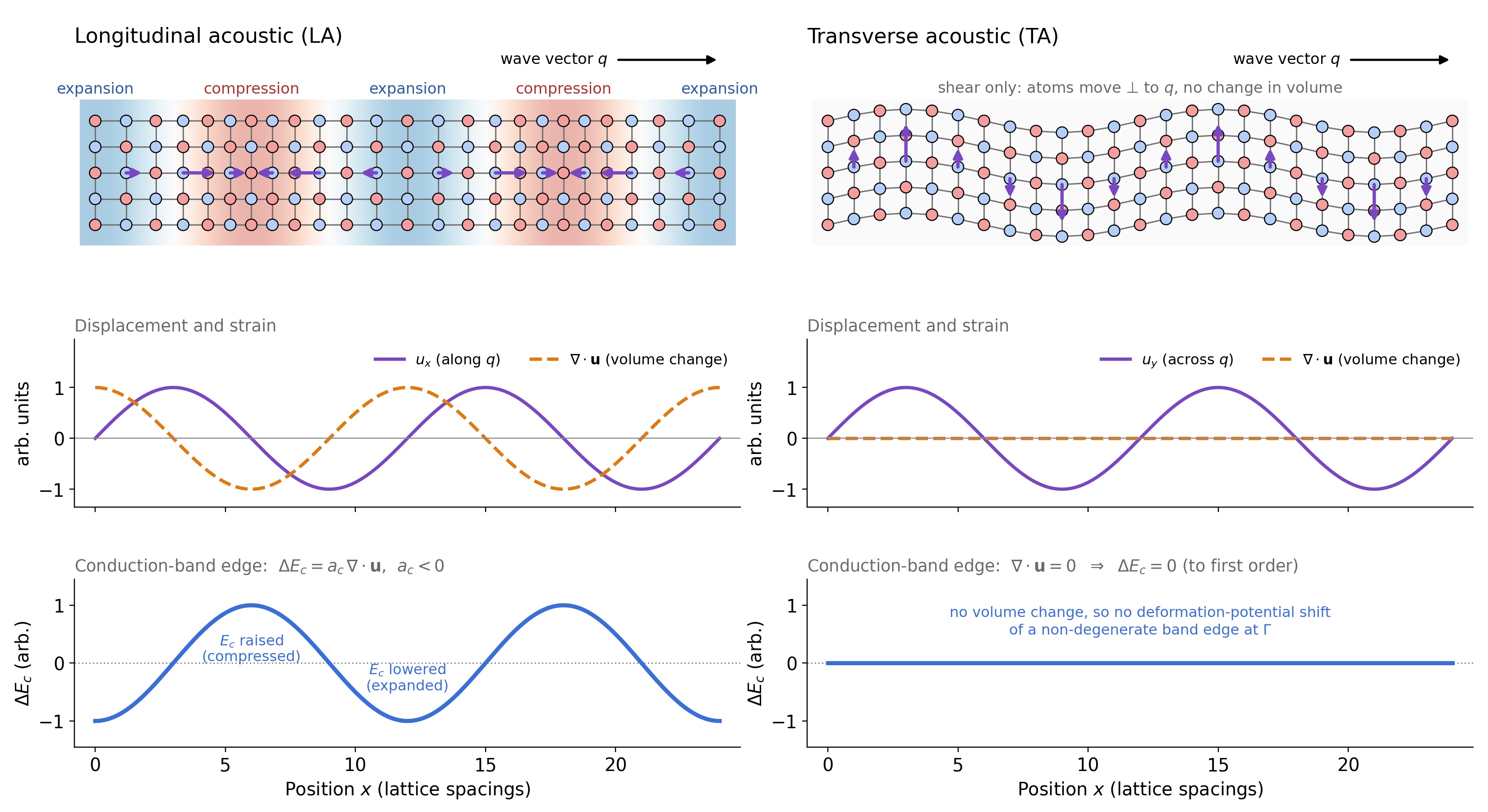
Why do these vibrations matter to an electron? Compressing, stretching or shearing a crystal slightly changes the environment experienced by its charge carriers. A travelling vibration therefore produces a moving disturbance in the semiconductor's electronic energies. An electron or hole interacting with that disturbance can change the direction in which it travels. This is called acoustic phonon scattering.

Scattering does not necessarily mean that a carrier loses much energy. Acoustic phonons often exchange only a small amount of energy with an electron, but they can still change its direction significantly. This matters because repeatedly changing direction makes it harder for carriers to move steadily through a device, reducing their mobility. Figure ?? later in this tutorial illustrates why a large change in direction affects mobility more strongly than a small one.

Acoustic phonons exist in materials such as silicon, GaAs and GaN, and they scatter carriers in both bulk semiconductors and quantum wells. They differ from the optical vibrations discussed in the Fröhlich scattering tutorial: acoustic waves are sound-like lattice motions whose energy becomes very small at long wavelengths. The sections below explain the physics quantitatively, starting with how deformation shifts the electronic band energies.

2. How a lattice vibration scatters a carrier

Acoustic phonons are sound-like waves: longer wavelengths correspond to lower vibration frequencies. Over sufficiently long wavelengths, their frequency is approximately proportional to their wavevector. The simplest acoustic scattering mechanism is deformation-potential coupling. When the lattice is compressed or stretched, the electronic band energies change. A passing acoustic wave therefore creates a spatially and temporally varying potential experienced by electrons and holes. For an isotropic band, this energy shift can be represented by

\[ \Delta E(\mathbf r,t)=D_{\mathrm{ac}}\,\nabla\!\cdot\mathbf u(\mathbf r,t) =D_{\mathrm{ac}}\,\mathrm{Tr}\,\boldsymbol\varepsilon(\mathbf r,t), \]

where \(\mathbf u\) is the lattice displacement, \(\boldsymbol\varepsilon\) is the strain tensor and \(D_{\mathrm{ac}}\) is the acoustic deformation potential, with units of energy. A longitudinal wave creates local compression and expansion, giving a nonzero strain trace. A purely transverse plane wave has zero strain trace, so it does not couple through this scalar hydrostatic term. This does not mean transverse acoustic phonons can never scatter carriers: anisotropic and multiband deformation potentials can also couple to shear strain.

More generally the symmetric strain tensor is

\[ \varepsilon_{ij}=\frac{1}{2} \left(\frac{\partial u_i}{\partial x_j}+\frac{\partial u_j}{\partial x_i}\right). \]

The strain-induced electronic Hamiltonian may contain several independent deformation potentials rather than a single constant. Such descriptions become important for anisotropic conduction-band valleys and valence bands with mixed orbital and spin character.

3. Phonon occupation and the elastic approximation

Acoustic phonons can change both the energy and direction of a carrier. Figure ?? illustrates these two effects before we introduce their mathematical description.

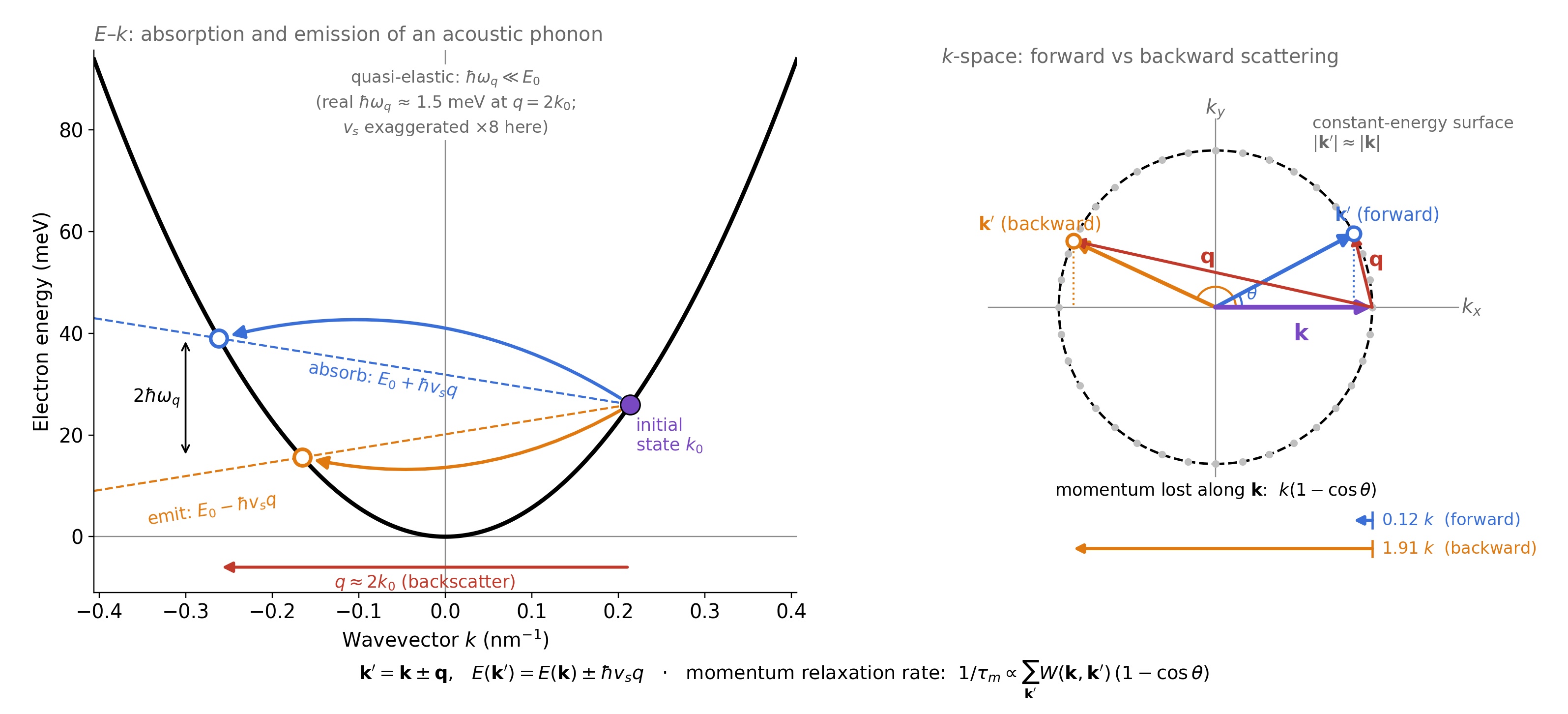
A carrier can absorb an acoustic phonon, gaining energy \(\hbar\omega_\lambda\), or emit one, losing the same energy. The mean number of phonons in a mode at lattice temperature \(T\) is given by the Bose–Einstein distribution:

\[ N_{\mathbf q\lambda}= \frac{1}{\exp[\hbar\omega_\lambda(\mathbf q)/(k_BT)]-1}. \]

Absorption is proportional to \(N_{\mathbf q\lambda}\), whereas emission is proportional to \(N_{\mathbf q\lambda}+1\). The extra unity represents spontaneous emission. At sufficiently high temperature for the phonons carrying most of the momentum transfer, \(k_BT\gg\hbar\omega_\lambda\), the occupation approaches

\[ N_{\mathbf q\lambda}\simeq\frac{k_BT}{\hbar\omega_\lambda(\mathbf q)}. \]

Acoustic phonon energies are often small compared with the relevant carrier energies, allowing the quasi-elastic, equipartition approximation \(E_f\simeq E_i\). Absorption and emission then contribute to transitions between approximately equal-energy electronic states. This is an approximation, not a statement that acoustic phonons carry no energy. It becomes less reliable at low temperature, at high phonon wavevector, or when the energy exchanged is comparable with the carrier energy.

4. Deformation-potential matrix element

In the isotropic, long-wavelength model a longitudinal acoustic phonon couples to a carrier through the deformation potential. For a plane-wave electronic state, the single-phonon coupling has the standard magnitude

\[ |M_{\mathbf q,\mathrm{LA}}|^2= D_{\mathrm{ac}}^2\frac{\hbar|\mathbf q|}{2\rho V v_{\mathrm{LA}}}, \]

where \(\rho\) is the mass density and \(V\) is the phonon normalisation volume. For more general electronic states the coupling also contains an overlap between the initial and final wavefunctions. The scattering strength therefore depends on both the lattice vibration and the electronic band character.

Combining phonon absorption and emission in the high-temperature quasi-elastic limit gives a particularly useful result for the isotropic longitudinal contribution:

\[ |M_{\mathrm{LA}}|^2_{\mathrm{thermal}} \simeq\frac{D_{\mathrm{ac}}^2 k_BT}{\rho V v_{\mathrm{LA}}^2} \,\mathcal F_{if}, \]

where \(\mathcal F_{if}\) denotes the appropriate electronic-state overlap factor. This expression shows why acoustic scattering normally becomes stronger as temperature increases. It also shows that the scattering depends on the deformation potential, crystal density and elastic response, not merely on an adjustable mobility parameter.

5. Longitudinal, transverse and anisotropic acoustic modes

Sound travels at different speeds along different crystallographic directions in many semiconductors. The acoustic frequencies and displacement polarisations follow from the crystal's elastic stiffness tensor \(C_{ijkl}\). In the continuum description they are found from the Christoffel equation:

\[ \sum_{j}\Gamma_{ij}(\hat{\mathbf q})e_j^{(\lambda)} =\rho v_\lambda^2 e_i^{(\lambda)}, \qquad \Gamma_{ij}(\hat{\mathbf q}) =\sum_{k,l} C_{ikjl}\hat q_k\hat q_l. \]

The eigenvalues determine the sound velocities, while the eigenvectors \(\mathbf e^{(\lambda)}\) determine the phonon polarisations. These polarisations specify which combinations of compression and shear are produced by each mode, and hence which deformation-potential couplings are possible.

For a cubic crystal, the elastic response is described by three independent stiffnesses, conventionally \(C_{11}\), \(C_{12}\) and \(C_{44}\). A hexagonal wurtzite crystal requires additional independent elastic constants, because the response along the crystal's \(c\)-axis generally differs from the response in the basal plane. Elastic anisotropy can therefore make scattering rates and mobility direction-dependent even before electronic-band anisotropy is considered.

6. Deformation potentials for different electronic bands

The scalar deformation potential is an instructive starting point, but real semiconductors can have multiple bands, valleys and wavefunction components. In these materials acoustic strain can shift, split or mix electronic states.

Conduction-band valleys in silicon: The response of a valley depends on its orientation. A common description separates a hydrostatic deformation potential \(\Xi_d\) from a uniaxial term \(\Xi_u\):

\[ \Delta E_{\nu}=\Xi_d\,\mathrm{Tr}\,\boldsymbol\varepsilon +\Xi_u\,\hat{\mathbf a}_{\nu}\!\cdot\boldsymbol\varepsilon\!\cdot\hat{\mathbf a}_{\nu}, \]

where \(\hat{\mathbf a}_{\nu}\) is the valley-axis unit vector. Strain can consequently affect valleys along different crystal axes differently.

Valence bands and multiband semiconductors: Heavy-hole, light-hole and spin-orbit-coupled states respond to shear and uniaxial strain, as well as hydrostatic strain. The Bir–Pikus strain Hamiltonian provides a standard description for zincblende and related multiband systems. The scattering probability between states \(|i\rangle\) and \(|f\rangle\) is controlled by a matrix element of the strain perturbation,

\[ M_{fi}^{(\lambda)}\propto \langle f|H_{\mathrm{strain}}(\boldsymbol\varepsilon^{(\lambda)})|i\rangle. \]

This form allows shear-induced coupling, band mixing and selection rules to influence the scattering probability. The relevant deformation potentials and strain Hamiltonian depend on the semiconductor's symmetry and band structure; one universal scalar constant cannot describe all such cases.

7. Acoustic scattering in quantum wells

In a quantum well, electronic motion is confined in the growth direction (taken here to be \(z\)), while carriers remain free to move in the plane. An electronic state can be written schematically as a product of an in-plane plane wave and a confined envelope wavefunction. Its response to an acoustic phonon depends on the overlap of the initial and final confined states.

For a scalar deformation potential, the relevant confinement factor has the form

\[ I_{fi}(q_z)=\int dz\,\psi_f^*(z) D_{\mathrm{ac}}(z)\psi_i(z)e^{iq_z z}. \]

Here \(q_z\) is the phonon wavevector component perpendicular to the well, and \(\psi_i\), \(\psi_f\) are confined electronic wavefunctions. The oscillatory factor represents the phonon's variation across the well. The same physical principle extends to multicomponent wavefunctions, where the scalar deformation potential is replaced by an appropriate strain Hamiltonian.

Acoustic phonons are three-dimensional vibrations even when the electronic states are two-dimensional. In the usual bulk-phonon description of a quantum well, a carrier can exchange an in-plane momentum \(\mathbf q_\parallel=\mathbf k'_\parallel-\mathbf k_\parallel\) while also coupling to an out-of-plane phonon component \(q_z\). This makes the confinement overlap important for both intrasubband and intersubband transitions. Alternative descriptions may be needed for freestanding membranes or other structures with strongly confined phonons.

8. From Fermi's golden rule to a scattering rate

The probability of a phonon-assisted transition follows from Fermi's golden rule. For an initial electronic state \(i\), the total scattering rate is obtained by summing over allowed final states, phonon branches and phonon wavevectors:

\[ \begin{aligned} \frac{1}{\tau_i} = \frac{2\pi}{\hbar} \sum_{f,\mathbf q,\lambda}|M_{fi}^{(\lambda)}(\mathbf q)|^2 \Big[&N_{\mathbf q\lambda}\, \delta(E_f-E_i-\hbar\omega_{\mathbf q\lambda})\\ &+(N_{\mathbf q\lambda}+1)\, \delta(E_f-E_i+\hbar\omega_{\mathbf q\lambda})\Big]. \end{aligned} \]

The first term describes absorption and the second emission. The Dirac delta functions enforce energy conservation; crystal momentum is conserved through the relationship between the electronic and phonon wavevectors. In degenerate systems, occupation of the final electronic states also matters, introducing Pauli-blocking factors.

In the high-temperature elastic approximation the two contributions approach a single equal-energy scattering process, with the thermal matrix element discussed above. For a general electronic dispersion \(E_b(\mathbf k)\), the available final states lie on the same-energy contour or surface:

\[ E_{b_f}(\mathbf k')=E_{b_i}(\mathbf k). \]

This emphasises an important distinction: acoustic scattering is influenced by the density and geometry of accessible electronic states, as well as the phonon coupling. Nonparabolic or anisotropic bands can therefore have energy-dependent scattering rates quite different from the familiar isotropic effective-mass result.

9. Scattering lifetime, transport lifetime and mobility

Not every collision is equally effective at reducing electrical current. A collision that barely changes the direction of travel may contribute to the total scattering rate but relax momentum only weakly. For an isotropic band, the distinction is often represented by a transport weighting:

\[ \frac{1}{\tau_{\mathrm{tr}}(\mathbf k)} =\sum_{\mathbf k'}W_{\mathbf k\rightarrow\mathbf k'} \bigl(1-\cos\theta\bigr), \]

where \(W_{\mathbf k\rightarrow\mathbf k'}\) is the transition rate and \(\theta\) is the scattering angle. Forward scattering has little effect on momentum relaxation, while backscattering contributes more strongly. For anisotropic or multiband materials, a full treatment of momentum or velocity relaxation can be more complicated than this simple angular factor.

In the elementary parabolic-band relaxation-time approximation the mobility is

\[ \mu=\frac{q\tau_{\mathrm{tr}}}{m^*}. \]

Real devices generally contain carriers at a range of energies and may have several occupied bands or subbands. The conductivity then involves the carrier distribution, group velocities and energy-dependent transport lifetime. Acoustic phonon scattering is one contribution among others, such as impurities, interface roughness and optical phonons, that can limit the final mobility. See the band-structure and mobility documentation for the broader context of semiconductor transport modelling.

10. When is the simple acoustic model insufficient?

The deformation-potential and equipartition approximations offer a valuable description of acoustic scattering, but their assumptions should be kept in mind. At low temperatures, the phonon population and the energy of the phonons that can scatter electrons must be treated carefully; the Bloch–Grüneisen regime can depart markedly from the high-temperature picture. Strong anisotropy, multiband coupling and quantum confinement can alter scattering selection rules. Other acoustic interactions, notably piezoelectric scattering in non-centrosymmetric crystals, arise from a different physical coupling and should not be confused with deformation-potential scattering.

The central result is that acoustic phonons scatter carriers by producing time-dependent lattice strain. The strength of the interaction depends on how electronic states respond to strain, how the crystal supports sound waves, which final carrier states are available, and how effectively each transition relaxes momentum. These principles apply to bulk semiconductors as well as to quantum wells and multiband electronic systems.