Simulation modes and simulation editors

1. Introduction

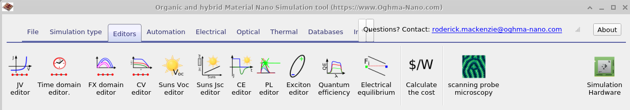
OghmaNano uses a modular, plugin-based architecture that applies the same core solver to many electrical and optical simulation types. Each plugin adapts the solver in a slightly different way—for example, one runs steady-state JV sweeps, another performs frequency-domain analysis, and another calculates external quantum efficiency (EQE). Every plugin is represented by an icon in the simulation editors ribbon (??), which you can click to open its editor and adjust the simulation parameters.

Editors ribbon with icons for JV, Time-domain, Frequency-domain, CV, Suns–Voc, Suns–Jsc, Charge extraction, Steady-state PL, Exciton, Quantum efficiency, Electrical equilibrium, and related tools. — Editors ribbon — click an icon to open its plugin and configure experiments for electrical or optical simulations.

2. Editing simulation modes

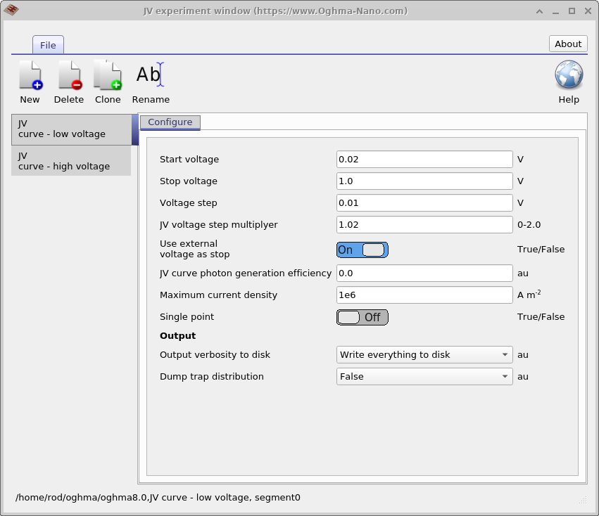
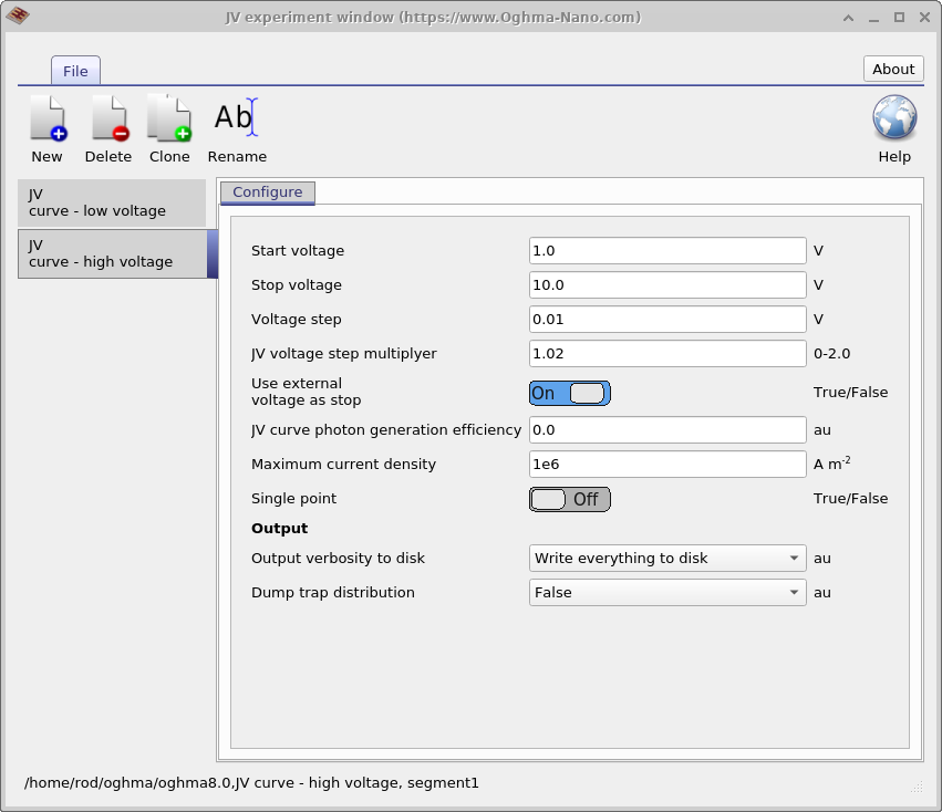
By clicking an icon in the simulation editors ribbon you can open the corresponding plugin editor and adjust how that simulation is performed. For example, in the JV editor you can set the start and stop voltages of a sweep. Two such setups are shown in ?? and ??: one experiment called JV curve – low voltage (0.02–1.0 V) and another called JV curve – high voltage (1.0–10.0 V). Each setup is referred to as an experiment — a saved configuration of simulation parameters within a plugin. Defining multiple experiments is especially useful in more complex cases, such as time-domain studies where you may want to test several voltage or light pulse profiles on the same device. There is no fixed limit to how many experiments you can create in each plugin.

JV editor showing an experiment ‘JV curve – low voltage’ with Start 0.02 V, Stop 1.0 V, Step 0.01 V, and step multiplier 1.02. — JV editor — low-voltage experiment (0.02–1.0 V). Multiple experiments of the same simulation type can live in one editor.

JV editor showing an experiment ‘JV curve – high voltage’ with Start 1.0 V, Stop 10.0 V, Step 0.01 V, and step multiplier 1.02. — JV editor — high-voltage experiment (1.0–10.0 V). Named experiments are saved simulation setups.

2. Running a simulation mode

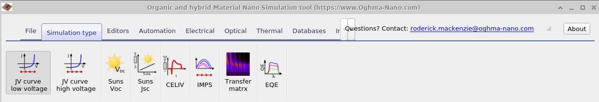
Once an experiment is defined, it appears as an icon in the simulation modes ribbon (??). In this example, the ribbon shows icons for both JV curve – low voltage and JV curve – high voltage, corresponding to the experiments defined in ?? and ??. The pressed (depressed) icon indicates the active mode — here, JV curve – low voltage. When you press the play button (or F9), only the selected mode is executed. At any time, exactly one simulation mode can be active.

Simulation type ribbon with selectable experiments: JV low voltage (selected), JV high voltage, Suns–Voc, Suns–Jsc, CELIV, IMPS, Transfer-matrix optics, and EQE. — Simulation modes ribbon — the pressed icon (*JV curve – low voltage*) is the experiment that will run when you press Play (`F9`).

4. All plugins

A list of the available plugins and what they do is given below:

Plugin	Description
`jv`	Calculate steady-state JV curves.
`suns_jsc`	Simulate Suns vs. J_sc curves.
`suns_voc`	Suns vs. V_oc simulations.
`eqe`	Simulate external quantum efficiency (EQE).
`cv`	Capacitance–voltage simulations.
`ce`	Simulate charge extraction experiments.
`time_domain`	Time-domain solver for transient simulations.
`fx_domain`	Simulate frequency-domain response (electrical and optical excitation).
`pl_ss`	Calculate photoluminescence (PL) spectrum in steady state.
`mode`	Solve optical modes in 1D/2D waveguides.
`spm`	Simulate scanning probe microscopy in 3D electrical simulations.
`equilibrium`	Equilibrium electrical simulations.
`exciton`	Exciton transport and recombination simulations.
`mesh_gen`	Generate meshes for simulations.